Machine Learning
Gaussian Process Classification
Classification Problem 분류 문제의 두 가지 관점 베이지안 관점에서 분류(Classification) 문제를 정의하는 과정을 생각해보면, 설명변수 $\mathbf{x}$와 반응변수(class) $y$의 결합확률분포 $p(y,\mathbf{x})$를 접근하는 방식에 두 가지 방법이 있음을 고려할 수 있다. $$ p(y,\mathbf{x}) = p(y)p(\mathbf{x...
Classification Problem
분류 문제의 두 가지 관점
베이지안 관점에서 분류(Classification) 문제를 정의하는 과정을 생각해보면, 설명변수 와 반응변수(class) 의 결합확률분포 를 접근하는 방식에 두 가지 방법이 있음을 고려할 수 있다.
두 번째 항과 세 번째 항 모두 조건부 분포를 정의하는 것에 의해 표현되며, 이때 두 접근 방법을 각각 generative approach, discriminative approach 라고 한다.
Generative approach
Generative approach에서는 class-conditional distribution 를 모델링하고, 각 class()에 대한 사전분포를 설정하여 다음과 같이 사후확률분포를 구한다.
Discriminative approach
반면, discriminative approach의 경우에는 response function 을 사용하여 설명변수가 주어질 때 각 클래스에 속할 확률을 모델링한다. 아래는 이러한 접근법을 사용한 예시로 선형 로지스틱 회귀모형을 나타낸다.
이번 포스팅에서 다룰 Gaussian Process를 이용한 분류 모형은 discriminative approach에 기반한 것이다.
Linear Classification
Gaussian Process Classifier를 다루기에 앞서, 우선 간단한 선형분류기를 살펴보도록 하자. 반응변수가 두 가지 클래스()를 갖고 다음과 같이 가능도함수가 주어진다고 하자.
또한, 주어진 분류 문제에서 데이터셋이 으로 주어지고, parameter 에 대한 가우시안 사전분포()를 정해주면 다음과 같은 로그사후확률분포를 구할 수 있다.
다만, 식으로부터 알 수 있다시피 회귀모형과는 다르게 MAP estimator의 closed form을 구할 수 없다. 대신 특정 response function(로지스틱, 정규분포 cdf)등을 사용했을 때 위 로그사후분포의 형태가 concave function이 되고, 이를 이용하면 Newton-Raphson 등을 이용해 추정량을 구할 수 있다.
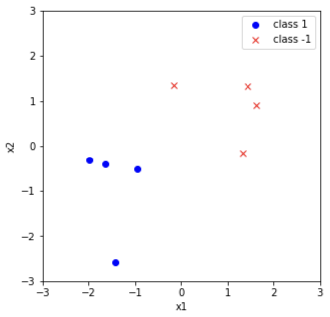
Example
-
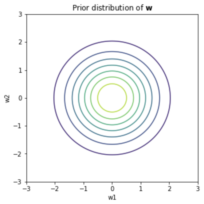
- Prior Distribution
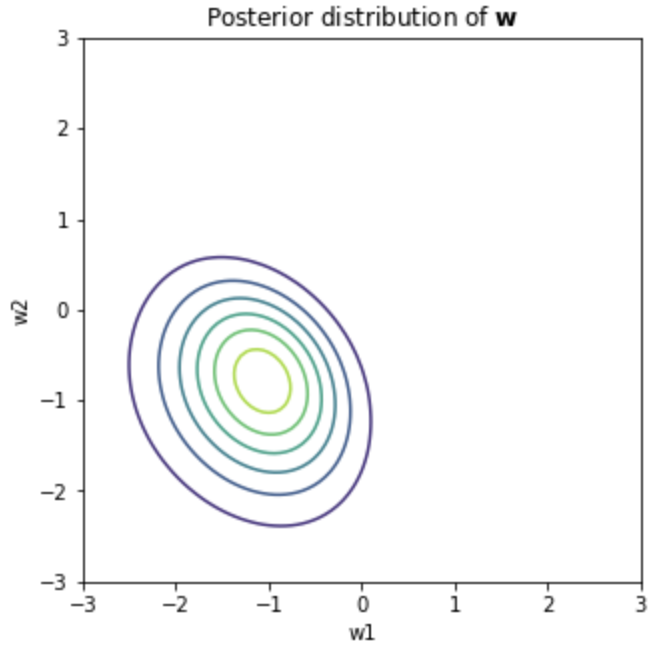
- Posterior Distribution
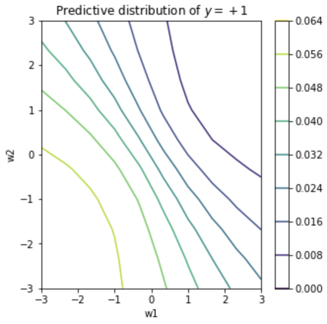
- Predictive Distribution
Gaussian Process Classification
분류 문제에서 Gaussian Process를 사용하는 것은 단지 latent function이라 하는 함수 에 대해 gaussian process 사전분포를 설정하는 것이다. 다만, 앞서 설명한 discriminative approach에서 도출해야 하는 것은 각 데이터들에 대한 클래스별 확률값(0과 1 사이)이므로, 로지스틱 함수와 같은 sigmoid를 거친 를 이용하게 된다. 계산의 편의를 위해 관측모형이 noise-free, 즉 로 noise term() 없이 직접 표현된다고 가정하자.
Inference
추론 과정은 우선 test data 에 대한 latent variable 의 확률분포를 계산하는 것으로부터 시작된다.
여기서 input data에 대한 latent variable 의 posterior distribution은 다음과 같다.
다음으로, 이를 이용하여 test data에 대한 예측 확률을 다음과 같이 계산할 수 있다.
Gaussian Process Regression의 경우와 다른 것은, posterior distribution
가 gaussian distribution이 아니므로, 가능도함수를 직접 계산하는 방식으로 추론 및 예측하는 것은 어렵다. 이를 위해 non-Gaussian joint posterior를 근사하기 위한 Laplace approximation, Expectation propagation 혹은 MCMC approximation 등이 사용된다.
References
- Gaussian Process for Machine Learning
- Code on Github