Archive
Spatio-Temporal Graph Convolutional Networks
Graph Convolutional Network는 Graph Neural Network의 가장 대표적인 모델 중 하나입니다. Graph Neural Network는 그래프 구조를 이용하여 노드의 특성을 업데이트하는 방법으로, 최근에는 다양한 분야에 적용되고 있습니다. 이번 글에서는 Graph Convolutional Network (GCN) 과 이를 시공간 데이터에 적용한 Spatio...
Graph Convolutional Network는 Graph Neural Network의 가장 대표적인 모델 중 하나입니다. Graph Neural Network는 그래프 구조를 이용하여 노드의 특성을 업데이트하는 방법으로, 최근에는 다양한 분야에 적용되고 있습니다.
이번 글에서는 Graph Convolutional Network (GCN) 과 이를 시공간 데이터에 적용한 Spatio-Temporal Graph Convolutional Networks (STGCN), 그리고 이에 Attention Mechanism을 추가한 Attention Based Spatial-Temporal Graph Convolutional Networks (ASTGCN) 에 대해 알아보겠습니다.
Graph Convolutional Network (GCN)
우선, GCN에 대해 살펴보도록 하겠습니다. GCN은 2017년에 Kipf와 Welling에 의해 제안된 논문에서 처음 소개되었습니다. GCN은 그래프 구조를 이용하여 노드의 특성을 업데이트하는 방법입니다.
개의 노드로 구성된 Graph (여기서 는 노드 집합, 는 엣지 집합) 가 주어졌을 때, graph Laplacian 은 다음과 같이 정의됩니다.
여기서 는 degree matrix로, 입니다. 는 adjacency matrix인접행렬로, 이면 노드 와 사이에 엣지가 존재함(connected)을 의미합니다. GCN은 이러한 그래프 구조를 이용하여 노드의 특성을 업데이트하는 방법입니다. 노드 의 특성을 라고 할 때, GCN은 다음과 같이 노드의 특성을 업데이트합니다. (여기서 특성이란 노드에 대응하는 변수들을 의미합니다.)
여기서 는 번째 레이어의 노드 특성을 의미하며, 는 self-loop를 추가한 adjacency matrix입니다. 는 에 대응하는 degree matrix입니다. 는 번째 레이어의 가중치 행렬이며, 는 활성화 함수(ReLU)입니다. 이러한 방식으로 GCN은 그래프 구조를 이용하여 노드의 특성을 업데이트합니다.
Spectral Graph Convolution
위 식 이 도출되는 과정은 spectral graph convolution이라는 연산을 이용하여 설명할 수 있습니다. Spectral graph convolution은 그래프 신호를 Fourier domain에서 다루는 방법입니다.
각 노드에 대해 스칼라 값으로 이루어진 신호 가 주어졌을 때, filter(혹은 kernel) 에 대한 graph convolution operator 는 다음과 같이 정의됩니다.
여기서 는 그래프 의 normalized graph Laplacian 의 eigenvector로 이루어진 행렬입니다. 는 의 eigenvalue에 대응하는 filter로, 입니다. 이러한 방식으로 spectral graph convolution은 그래프의 eigenvector를 이용하여 노드의 특성을 업데이트합니다.
Chebyshev Polynomial Approximation
다만, 식 는 계산량이 매우 크다는 문제점이 있습니다 (). 이를 해결하기 위해 Kipf와 Welling은 Chebyshev polynomial approximation을 이용하여 spectral graph convolution을 근사하는 방법을 제안했습니다. 이는 다음과 같이 정의됩니다.
즉, kernel 를 차까지의 Chebyshev polynomial 로 근사하는 것입니다. Chebyshev polynomial은 다음과 같이 재귀적으로 정의됩니다.
이를 이용하면, graph convolution operator는 다음과 같이 근사될 수 있습니다.
여기서 는 normalized graph Laplacian 을 이용하여 정의한 것입니다. 이러한 방식의 근사는, 계산 비용을 로 줄일 수 있습니다.
Layer-wise Propagation
위의 spectral graph convolution (식 )을 기반으로 neural network를 구성할 수 있습니다. 우선, 식 를 로 설정하면, 다음과 같이 나타낼 수 있습니다.
또한, 나아가 로 설정하면, 가 됩니다. 이를 이용하면, 식 는 다음과 같이 나타낼 수 있습니다.
이때 두 개의 parameter 과 을 이용하여 노드의 특성을 업데이트할 수 있습니다. 또한, 이를 더 간단히 하여 로 설정하면, 다음과 같이 나타낼 수 있습니다.
로 설정하였기 때문에 의 eigenvalue는 사이에 있습니다. 또한, 위 연산자 을 반복적으로 사용할 경우 gradient vanishing/exploding 문제가 발생할 수 있습니다. 이를 해결하기 위해 Kipf와 Welling은 다음과 같은 renormalization trick을 제안하였습니다.
이를 일반화하여, signal matrix 에 대해 다음과 같이 노드의 특성을 업데이트할 수 있습니다 (차원 feature vector). 이것이 바로 GCN의 layer-wise propagation 방식입니다. (식 )
는 가중치 행렬이며, 출력 행렬은 입니다. 이러한 방식의 계산은 총 의 계산량을 가지며, 이를 이용하여 GCN을 구성할 수 있습니다.
PyTorch Implementation
Graph convolution layer를 PyTorch로 구현하면 다음과 같습니다.
import torch
import torch.nn as nn

class GraphConvolution(nn.Module):
    def __init__(self, in_features, out_features):
        super(GraphConvolution, self).__init__()
        self.in_features = in_features
        self.out_features = out_features
        self.weight = nn.Parameter(torch.FloatTensor(in_features, out_features))
        self.reset_parameters()

    def forward(self, input, adj):
        support = torch.mm(input, self.weight)
        output = torch.spmm(adj, support)
        return output

    def reset_parameters(self):
        nn.init.xavier_uniform_(self.weight)
forward 메소드에서는 입력 input과 adjacency matrix adj를 이용하여 노드의 특성을 업데이트합니다. 이때 input은 노드의 특성을 나타내는 행렬이며, adj는 adjacency matrix입니다. reset_parameters 메소드에서는 가중치 행렬을 초기화합니다. 또한, torch.spmm은 sparse matrix와 dense matrix의 곱을 계산하는 함수입니다. 이를 이용하여 GCN을 구성할 수 있습니다.
import torch
import torch.nn as nn

class GCN(nn.Module):
    def __init__(self, in_features, hidden_features, out_features):
        super(GCN, self).__init__()
        self.gc1 = GraphConvolution(in_features, hidden_features)
        self.gc2 = GraphConvolution(hidden_features, out_features)

    def forward(self, x, adj):
        x = F.relu(self.gc1(x, adj))
        x = self.gc2(x, adj)
        return x
Spatio-Temporal Graph Convolutional Networks (STGCN)
이제 STGCN에 대해 알아보도록 하겠습니다. STGCN은 B. Yu, H. Yin, and Z. Zhu에 의해 2018년에 제안된 논문에서 처음 소개되었습니다. STGCN은 GCN을 시공간 데이터에 적용한 방법입니다. 이 논문에서는 교통량 예측에 STGCN을 적용하여 좋은 성능을 보였습니다.
STGCN Structure
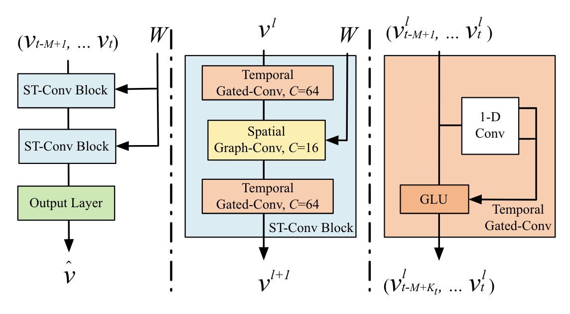 STGCN Structure (Source: B. Yu, H. Yin, and Z. Zhu, 2018)
교통량 예측은 각 도로에 대해 일정 시간 간격으로 측정된 교통량 데이터를 이용하여 미래의 교통량을 예측하는 문제입니다. 이전 시점의 교통량을 이용하여 시점까지의 교통량을 예측하는 문제를 고려해보도록 하겠습니다. 전체 노드의 개수를 이라고 하고 (여기서는 도로가 노드에 해당합니다) 을 시점 의 각 노드의 교통량을 나타내는 벡터라고 하겠습니다. 그러면, 교통량 예측 문제는 다음과 같이 정의됩니다.
공간적인 특성을 고려하는 것은 앞서 살펴본 GCN을 이용하여 풀 수 있습니다. 다만 시간적인 특성을 고려하는 것 역시 중요한데, 이를 해결하기 위해 STGCN에서는 Temporal Gated Convolution을 사용합니다.
Temporal Gated Convolution
위 그림의 오른쪽 부분을 살펴보면 Temporal Gated Convolution이라는 구조를 볼 수 있습니다. Temporal convolution layer는 다음과 같이 정의됩니다.
식 의 의미를 살펴보도록 하겠습니다. 우선, temporal convolution 연산은 너비가 인 kernel을 이용한 1D convolution과 gated linear unit (GLU)를 이용합니다. 이때, 1D convolution 연산은 padding을 이용하지 않아, 개의 input은 개의 output을 생성합니다.
즉, 각 노드에 대한 temporal convolution의 input이 라면 convolution kernel은 이며, output은
입니다. 이때, 는 input feature의 차원, 는 output feature의 차원입니다. 또한, 는 각각 차원의 channel을 가집니다.
식 에서 는 sigmoid 함수이며, 는 element-wise productHadamard product을 의미합니다. 따라서, Temporal Gated Convolution은 1D convolution으로 두 개의 output 를 생성하고 이를 element-wise product하여 최종 output을 도출합니다.
Spatio-Temporal Convolution
이제, spatial convolution과 temporal convolution을 결합하여 Spatio-Temporal ConvolutionST-Conv을 정의할 수 있습니다. (위 그림의 2번째) 우선, 시공간성을 모두 고려해야 하므로 input, output은 모두 3D tensor로 정의됩니다.
번째 ST-Conv block에 대한 Input tensor 는 개의 노드, 개의 시점, 개의 feature로 이루어진 tensor입니다. 이때 output tensor는 다음과 같이 계산됩니다.
2개의 temporal convolution layer와 1개의 graph convolution layer를 이용하여 ST-Conv을 구성합니다. 이러한 조합을 ST-Conv block이라고 부르며, STGCN은 2개의 ST-Conv block과 1개의 fully connected layer로 구성됩니다 (위 그림의 왼쪽).
Attention Based Spatial-Temporal Graph Convolutional Networks (ASTGCN)
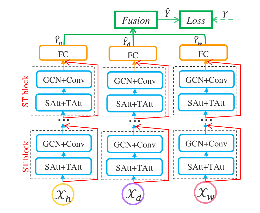
ASTGCN Structure (Source: S. Guo, Y. Lin, N. Feng, C. Song, and H. Wan, 2019)
ASTGCN은 Attention Mechanism을 이용하여 STGCN을 개선한 방법입니다. 위 그림처럼 세 개의 동일한 네트워크를 학습하는데, 각각의 네트워크는 recent, daily-periodic, weekly-periodic pattern을 학습합니다. 이를 Fusion layer를 이용하여 결합하여 예측 결과를 도출합니다. 데이터가 수집된 주기를 라고 하고, 예측할 시간 단위를 라고 하겠습니다.
-
Recent segment는 최근 시간 단위의 데이터를 이용합니다. Input tensor는 이며, 은 노드의 개수, 는 feature의 개수, 는 시간 단위입니다. 는 다음과 같이 주어집니다.
-
Daily-periodic segment는 일별 주기성을 학습합니다. Input tensor는 이며, 는 일 단위입니다. 는 다음과 같이 주어집니다.
여기서 는 샘플링이 이루어진 빈도를 의미하며, 는 예측할 시간 단위입니다 (식 ).
-
Weekly-periodic segment는 주별 주기성을 학습합니다. Input tensor는 이며, 는 주 단위입니다. 는 다음과 같이 주어집니다.
위와 같이, daily-periodic segment와 weekly-periodic segment는 각각 일별, 주별 주기성을 학습합니다. 또한, 위 정의에 따라 는 모두 의 배수가 되어야 합니다. 다음 그림을 참고하면, 각 segment의 구조를 쉽게 이해할 수 있습니다.
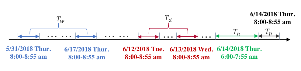 Recent, Daily, Weekly segment (Source: S. Guo, Y. Lin, N. Feng, C. Song, and H. Wan, 2019)
Spatial-Temporal Attention Mechanism
ASTGCN에서 핵심이 되는 아이디어는 Spatial-Temporal Attention Mechanism입니다. 각 노드가 다른 노드에 미치는 영향을 고려하기 위해 Attention Mechanism을 이용합니다.
우선, Spatial attention은 다음과 같이 정의됩니다.
여기서 은 번째 spatial-temporal block의 input tensor이며, 은 이전 block의 feature 차원을, 은 이전 block의 시간 길이를 의미합니다. 인 경우 은 recent, daily-period, weekly-period component에서 각각 를 의미합니다.
는 학습 가능한 parameter입니다. 는 활성화 함수로, 여기서는 sigmoid 함수를 사용합니다. 는 spatial attention matrix로, 각 노드가 다른 노드에 미치는 영향을 나타냅니다.
이를 통해 계산한 를 spatial attention matrix 라고 부르며, 이것에 softmax 함수를 적용하여 spatial attention matrix를 정규화합니다. 는 노드 와 노드 의 correlation을 나타냅니다.
Temporal Attention Mechanism
다음으로, Temporal attention 역시 유사하게 정의할 수 있습니다.
Matrix 는 temporal attention matrix로, 이는 두 시점 간의 correlation을 나타냅니다.
Fusion Layer
마지막 단계에서는 세 개의 segment에서 얻은 정보를 결합하여 예측 결과를 도출합니다. 이를 위해 Fusion layer를 이용합니다. 이는 세 개의 learable weight matrix 를 이용하여 다음과 같이 계산됩니다.
References
- B. Yu, H. Yin, and Z. Zhu, “Spatio-Temporal Graph Convolutional Networks: A Deep Learning Framework for Traffic Forecasting,” in Proceedings of the Twenty-Seventh International Joint Conference on Artificial Intelligence, Jul. 2018, pp. 3634–3640. doi: 10.24963/ijcai.2018/505.
- S. Guo, Y. Lin, N. Feng, C. Song, and H. Wan, “Attention Based Spatial-Temporal Graph Convolutional Networks for Traffic Flow Forecasting,” Proceedings of the AAAI Conference on Artificial Intelligence, vol. 33, no. 01, Art. no. 01, Jul. 2019, doi: 10.1609/aaai.v33i01.3301922.
- T. N. Kipf and M. Welling, “Semi-Supervised Classification with Graph Convolutional Networks.” arXiv, Feb. 22, 2017. doi: 10.48550/arXiv.1609.02907.