Archive
Cox Process with Hamiltonian Monte Carlo
Cox Process Point Pattern 데이터를 모델링하는 일반적인 방법은 intensity function을 추정하는 것이다. 이때, intensity function이 $\lambda(x)=2\exp(-x)$ 와 같은 함수 형태로 주어질 수도 있지만, 이러한 함수를 직접 추정하는 것 대신 함수의 형태에 대해서도 추가적인 랜덤성을 가정하는 것이 가능하다. 이러한 방법을 Cox...
Cox Process
Point Pattern 데이터를 모델링하는 일반적인 방법은 intensity function을 추정하는 것이다. 이때, intensity function이 와 같은 함수 형태로 주어질 수도 있지만, 이러한 함수를 직접 추정하는 것 대신 함수의 형태에 대해서도 추가적인 랜덤성을 가정하는 것이 가능하다. 이러한 방법을 Cox Process라고 한다. 이번 글에서는 Cox process에 대한 정의와 log Gaussian Cox process를 Hamiltonian Monte Carlo로 추정하는 방법에 대해서 다루고자 한다.
Definition
Cox process는 intensity function 를 random process로 가정한다. Point process 가 에서 정의되어 있을 때, 가 Cox process라면 random intensity process 가 존재하여 다음과 같은 조건을 만족한다.
다만 가 어떤 분포를 따르는지에 대해서는 추가적인 가정이 필요하다. 가장 일반적인 가정은 가 Gaussian process를 따른다는 것이다. 이러한 가정을 **Log Gaussian Cox Process (LGCP)**라고 한다. 즉, 실변수 Gaussian process 가 존재하여 이다.
LGCP
LGCP가 stationary, isotropic이라고 가정하면 이는 mean function 와 covariance function 로 유일하게 결정된다. Isotropic LGCP의 경우, covariance function은 다음과 같이 정의된다.
여기서 은 correlation function이라고 하는데, 대표적인 correlation function으로는 exponential, Matern 등이 있다.
이러한 가정하에서, 개의 지점 에서의 가능도는 다음과 같이 주어진다.
HMC for LGCP
LGCP 의 가능도를 직접 최대화하는 것은 어렵기 때문에, 베이지안 방법을 사용하여 posterior distribution을 추정하는 것이 일반적이다. 또한, 모델 학습을 수행하기 위해서는 Gaussian process의 realisation을 고려해야 한다. 이를 위해 주어진 공간 도메인 을 일정한 격자로 나누고 각 격자에서의 intensity를 추정하는 방법을 사용한다.
주어진 도메인 를 개의 격자로 나누고, 각 지점의 중심점을 라고 하자. 각 격자에서의 log intensity는 로 나타낼 수 있고, 결합분포는
이다. 이때, 은 개의 1로 이루어진 벡터이고, 는 의 covariance matrix이다. 파라미터를 로 나타내면, log likelihood는 다음과 같이 주어진다.
여기서 이고, 는 번째 격자에서의 관측된 점의 개수이다. 는 각 격자의 넓이를 의미한다.
이로부터 log posterior는 다음과 같이 주어진다.
HMC
앞서 주어진 log posterior를 직접 최대화하는 것은 어렵기 때문에, 베이지안 추론에서는 사후분포를 근사하는 방법을 사용한다. VB, MCMC 등 다양한 방법이 존재하지만 여기서는 MCMC 중 Hamiltonian Monte Carlo를 사용하여 사후분포를 추정하는 방법을 다루고자 한다.
HMC는 Metropolis-Hastings 알고리즘을 개선한 방법으로, 파라미터들이 높은 상관성을 가질 때 특히 효과적이다. HMC는 (물리학에서 비롯된) Hamiltonian dynamics를 사용하여 파라미터 공간을 탐색하는데, 이때 Hamiltonian은 다음과 같이 주어진다.
Hamiltonian
를 각각 momentum운동량과 position위치으로 정의하자. 이때, Hamiltonian은 다음과 같이 주어진다.
여기서 는 potential energy, 는 kinetic energy로 정의된다. 이러한 Hamiltonian이 사용될 수 있는 근거는, 베이지안 추론에서 를 사후분포로 사용하고, 를 파라미터로 사용할 수 있기 때문이다.
물리학에서는 위치에너지를 중력에 의한 것으로 생각하고, 운동에너지를 입자의 움직임에 의한 것으로 생각한다. 통계학에서는 위치에너지를
와 같이 (unnormalized) log distribution으로 정의하고, 운동에너지는
와 같이 정의한다. 이때, 은 inverse mass matrix라고 부르며 이는 positive definite matrix이다.
Hamilton's Equations
Hamiltonian dynamics는 다음과 같은 미분방정식으로 주어지는데, 이를 Hamilton's equations라고 한다.
에너지 보존 법칙과 유사하게 Hamiltonian은 시간에 대해 불변인데, 이는 다음과 같이 확인할 수 있다.
Leapfrog Integration
Discrete한 시점 에서 Hamiltonian dynamics를 풀기 위해 leapfrog integration을 사용한다. 이는 일반적으로 미분방정식을 풀기 위해 사용되는 Euler method를 개선한 방법으로, 다음과 같이 주어진다.
즉, momentum을 반스텝만큼 업데이트하고, position을 한스텝만큼 업데이트한 후, momentum을 다시 반스텝만큼 업데이트한다. 이러한 과정을 반복하면, Hamiltonian dynamics를 풀 수 있다.
HMC Algorithm
앞선 내용을 바탕으로 MCMC 샘플러를 구성할 수 있다. 이때 일반적인 MCMC와는 달리 샘플링이 이루어지는 모수 공간이 차원인 공간임에 주의해야 한다.
Target distribution은 다음과 같다.
이때 관심 대상인 에 대한 주변분포는 다음과 같이 주어진다.
이전 단계의 state가 이라고 하자. 이때, 다음 단계의 state를 라고 하면, 다음과 같은 과정을 거친다.
-
Initial position 을 설정하고, momentum 를 random하게 설정한다.
q = q0 p = np.random.normal(0, 1, q.shape) -
Leapfrog integration을 사용하여 Hamiltonian dynamics를 풀고, 새로운 state 를 얻는다.
for i in range(L): p = p - 0.5 * epsilon * grad_U(q) q = q + epsilon * p p = p - 0.5 * epsilon * grad_U(q) -
Metropolis-Hastings 알고리즘을 사용하여 새로운 state를 accept/reject한다. 이때 acceptance probability는 다음과 같이 주어진다.
current_U = U(q0) current_K = 0.5 * np.sum(p**2) proposed_U = U(q) proposed_K = 0.5 * np.sum(p**2) alpha = np.exp(current_U - proposed_U + current_K - proposed_K) if np.random.uniform() < alpha: q0 = q -
Step 2-3을 반복하여 샘플을 얻는다.
위 알고리즘에서 알 수 있듯이, leapfrog steps , step size , mass matrix 등은 hyperparameter로 설정해야 한다. 이때, 이러한 hyperparameter들은 적절한 값을 찾기 위해 tuning이 필요하다.
Python Implementation
Python에서는 pymc 패키지를 사용하여 HMC를 구현할 수 있다. 패키지의 자세한 사용법은 이전 글을 참고하면 된다.
Data
예시에서 사용할 데이터는 pysal 패키지의 내장 데이터셋인 vautm17n을 사용한다. 데이터는 다음과 같이 로드할 수 있다.
# Packages
import pymc as pm
import libpysal as ps
import numpy as np
import matplotlib.pyplot as plt
import geopandas as gpd
import shapely
# Load data
f = ps.examples.get_path('vautm17n_points.shp')
fo = ps.io.open(f)
data = gpd.GeoSeries.from_file(f)

# Window size
print(data.total_bounds)
# [ 273959.66438135 4049220.9034143   972595.98957796 4359604.85977962]

# Plot data
data.plot()
plt.axis('off')
plt.show()
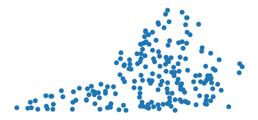
Data Points
추론을 위해서는 주어진 공간을 격자로 나누어야 한다. 예시에서는 격자 크기를 30000으로 설정하였다.
# Equally spaced grid

xmin, ymin, xmax, ymax = data.total_bounds
resolution = 30000

grid_cells = []

for x in np.arange(xmin, xmax, resolution):
    for y in np.arange(ymin, ymax, resolution):
        grid_cells.append(shapely.geometry.box(x, y, x + resolution, y + resolution))

grid = gpd.GeoDataFrame({'geometry': grid_cells})

# Plot grid
ax = grid.boundary.plot(figsize=(10, 10), linewidth=0.5)
data.plot(ax=ax, color='red', markersize=5)
plt.axis('off')
plt.show()
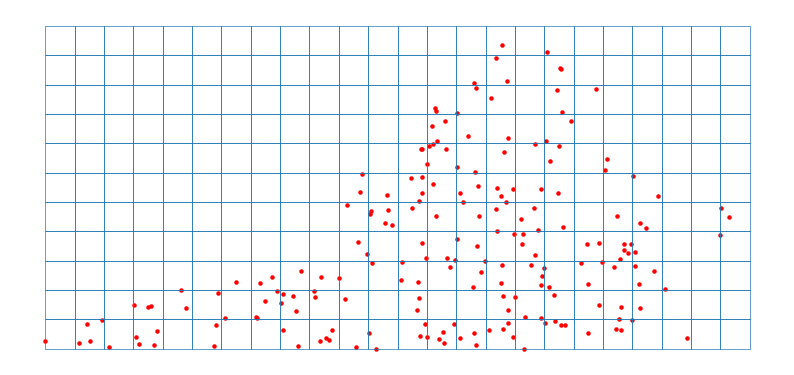 Data points and Grid
다음과 같이 각 격자에서의 점의 개수를 구할 수 있다. 또한, 이를 pymc에서 사용할 수 있게 numpy array로 변환한다.
# Count points in each grid cell
grid['cnt'] = 0
merged = gpd.sjoin(gpd.GeoDataFrame(data), grid, how='inner', op='within')
dissolve = merged.dissolve(by='index_right', aggfunc='count')
grid.loc[dissolve.index, 'cnt'] = dissolve['cnt']

centroids = grid.centroid.get_coordinates().to_numpy()
observed = grid['cnt'].to_numpy()
Model
pymc에서는 NUTS sampler를 사용하여 HMC를 구현할 수 있는데, 이는 HMC에서 step size와 leapfrog steps를 자동으로 설정해준다는 장점이 있다.
다음과 같이 모델을 구현할 수 있다.
with pm.Model() as lgcp_model:
    mu = pm.Normal('mu', sigma=1.0)
    rho = pm.Uniform('rho', lower=1000, upper=100000) # length scale
    variance = pm.InverseGamma('variance', alpha=1, beta=1)
    cov_func = variance * pm.gp.cov.Matern52(2, rho)
    mean_func = pm.gp.mean.Constant(mu)

    gp = pm.gp.Latent(mean_func=mean_func, cov_func=cov_func)
    log_intensity = gp.prior('log_intensity', X=centroids) # evaluate the GP at the centroids
    intensity = pm.math.exp(log_intensity)

    rates = intensity * resolution**2 / 1000000
    cnt = pm.Poisson('count', mu=rates, observed=observed)
Matern52 covariance function을 사용하였고, mu, rho, variance를 hyperparameter로 설정하였다. 이후, gp.prior를 사용하여 Gaussian process를 구현하였다.
Inference
다음과 같이 NUTS sampler를 사용하여 사후분포를 추정할 수 있다.
# Sample with HMC

with lgcp_model:
    trace = pm.sample(1000, tune=1000, cores=4, target_accept=0.95, progressbar=True)
여기서는 target_accept를 0.95로 설정하였는데, 이는 MH algorithm에서의 acceptance rate를 0.95로 유지하기 위한 hyperparameter이다. 코어 4개로 4개의 체인을 학습하였는데, 로컬 환경에서 대략 1시간 정도의 학습 시간이 소요되었다.
Results
 Trace Plot
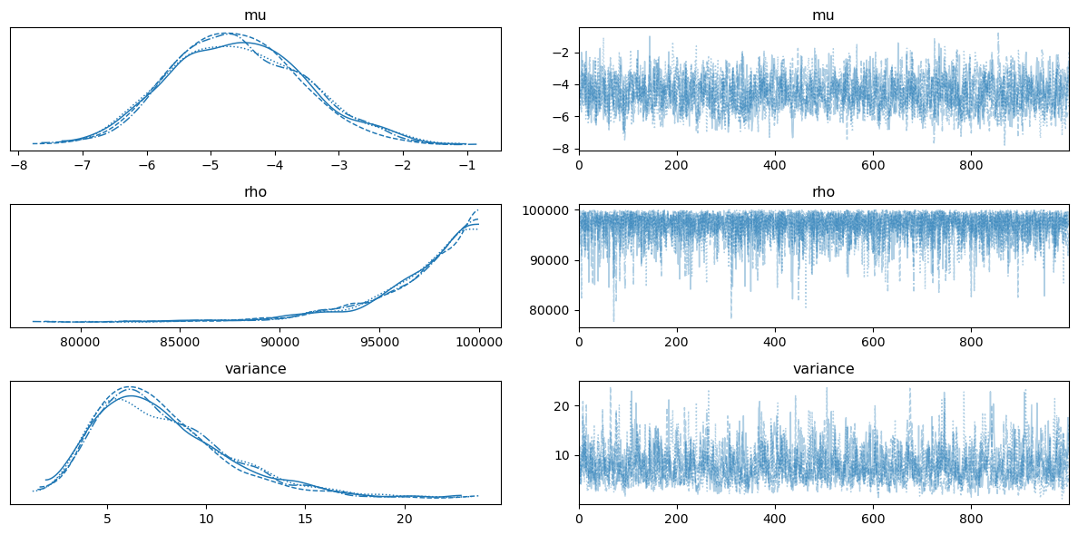
다음 코드로 hyperparameter 에 대한 사후분포를 확인할 수 있다. (위 그림 참고)
pm.plot_trace(trace, var_names=['mu', 'rho', 'variance'])
plt.tight_layout()
plt.show()
Lengthscale 의 경우 의 범위를 주었는데, MAP가 근방인 것으로 보아 범위를 더 크게 주어 학습시키는 것이 바람직할 것으로 보인다.
또한, 다음 코드로 log intensity 에 대한 사후 평균(posterior mean)을 구하고 이를 바탕으로 intensity plot을 그릴 수 있다.
# Posterior mean
posterior_mean = pm.find_MAP(model=lgcp_model, vars=[log_intensity])
intensities = np.exp(posterior_mean['log_intensity'])

# Plot intensities
grid['intensity_MAP'] = intensities
ax = grid.plot(column='intensity_MAP', figsize=(10, 5), legend=True, cmap='Blues')
data.plot(ax=ax, color='red', markersize=5)
grid.boundary.plot(ax=ax, linewidth=0.5)
plt.axis('off')
plt.tight_layout()
plt.show()
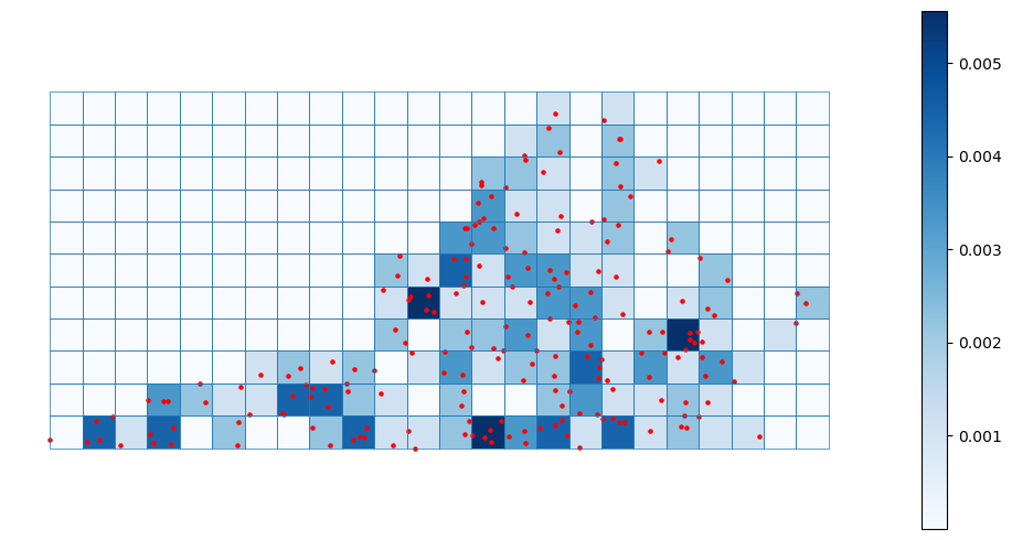 Posterior mean Intensities
References
- Møller, Jesper, Anne Randi Syversveen, and Rasmus Plenge Waagepetersen. 1998. “Log Gaussian Cox Processes.” Scandinavian Journal of Statistics 25 (3): 451–82.
- Teng, \Sigma., Nathoo, F. S., & Johnson, T. D. (2017). Bayesian Computation for Log-Gaussian Cox Processes: A Comparative Analysis of Methods. Journal of Statistical Computation and Simulation, 87(11), 2227–2252. https://doi.org/10.1080/00949655.2017.1326117
- Murphy, K. P. (2023). Probabilistic machine learning: Advanced topics. The MIT Press.