Archive
Differentially Private Variational Inference
Variational Inference with DP 이번 글에서는 다음 두 논문 - Jälkö, J. et al., (2017). Differentially Private Variational Inference for Non-conjugate Models - Wang, Y. et al., (2015). Privacy for Free: Posterior Sampling and Stoch...
Variational Inference with DP
이번 글에서는 다음 두 논문
- Jälkö, J. et al., (2017). _Differentially Private Variational Inference for Non-conjugate Models
- Wang, Y. et al., (2015). Privacy for Free: Posterior Sampling and Stochastic Gradient Monte Carlo.
논문 등을 바탕으로 Variational Inference 프레임워크에 DPDifferential Privacy가 어떻게 적용될 수 있는지 살펴보고자 한다. 또한, 이를 Python으로 구현하여 시뮬레이션을 수행해보았다.
Differential Privacy
DP에 대한 기본적인 정의는 이 글을 참고하면 좋을 것 같다.
Definition and Properties
Randomized algorithm 이 -DP를 만족한다는 것은 모든 가측집합 와 이웃하는 데이터셋 에 대해
를 만족하는 것을 말한다. -DP는 유용한 성질들이 있는데, 대표적인 두 가지는 다음과 같다.
Post-processing Immunity
이 -DP 인 알고리즘이면, 임의의 함수 에 대해 역시 -DP 이다.
Composition rule
이 -DP 이고, 가 -DP 라면 는 -DP 를 만족한다.
Posterior sampling
데이터 들이 주어질 때 모델 (parametric model의 경우는 모수를 의미)의 사후분포는 다음과 같이 주어진다.
One-Posterior Sample preserves DP
사후분포로부터 모델을 샘플링하는 것을 일종의 randomized algorithm으로 생각할 수 있을 것이다. 그렇다면 이에 대한 -DP를 고려할 수 있는데, 이에 대해서는 다음과 같은 정리가 성립한다.
-
로그가능도가 다음을 만족하면 (유계)
사후분포 로부터의 샘플링 는 -DP를 만족한다.
-
의 정의역이 유계이고 (i.e. ) 로그가능도가 -lipschitz 라면 샘플링 는 -DP를 만족한다.
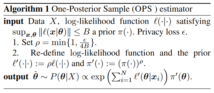
이로부터 다음과 같은 알고리즘을 구성할 수 있다.
OPS algorithm. Wang et al., 2015
OPS 샘플링은 consistency와 asymptotic normality도 갖는다. (자세한 내용은 논문 참고)
Variational Bayes
Variational Bayes 방법론은 ELBO로 부르는 evidence lower bound를 최대화하는 방향으로 학습하여 사후분포 를 variational distribution 로 근사한다.
Doubly stochastic variational inference
ELBO 을 계산하기 위해서는 부분의 계산이 요구된다. 적분을 계산하기 위해 Monte Carlo 샘플링을 사용할 수 있고, 구체적으로 라면 다음과 같이 샘플링을 수행할 수 있다.
이러한 방법을 doubly stochastic variational inference라고 한다. 이를 reparameterization trick이라고도 하는데, 자동 미분(automatic differentiation, AD)를 사용하는 SGD 알고리즘에는 이러한 방법이 필요하다 (ADVIAutomatic Differentiation Variational Inference 등).
DPVI
DPVI는 Variational Inference에 DP를 적용한 방법이다. 기본적으로 Deep Learning with Differential Privacy에서 다룬 gradient clipping 방법을 사용할 수 있고, 이를 Variational Inference에 적용한다. 전반적인 알고리즘은 다음과 같다.
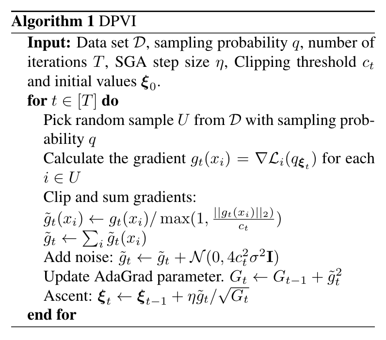 DPVI Algorithm
DPVI에서 샘플링 빈도 , 반복횟수 와 노이즈의 분산을 결정하는 은 privacy cost를 결정하는 중요한 파라미터들이다. 이에 대해 Abadi et al. 은 다음과 같은 정리로 -DP와의 관계를 보였다.
상수 가 존재하여, 샘플링 비율 과 스텝 수 가 주어졌을 때, 임의의 에 대해 DP-SGD를 사용하는 알고리즘은 아래 조건 하에서 -DP를 만족한다.
DPVI 알고리즘은 기본적으로 그래디언트 기반의 학습을 진행하기 때문에, 자동 미분이 가능한 환경에서 ELBO를 구현할 수 있다.
Python Implementation
DP-SGD 알고리즘을 포함하여, 앞서 살펴본 DPVI 알고리즘을 pytorch 기반으로 구현해보았다. 전체 코드는 다음 링크에서 확인가능하다.
우선 사용한 패키지들은 다음과 같다.
import numpy as np
import matplotlib.pyplot as plt
import pandas as pd
from sklearn.model_selection import train_test_split
from sklearn.datasets import load_breast_cancer
from sklearn.preprocessing import StandardScaler
import torch
from torch.distributions import Normal, Gamma
from torch.nn import Module, Parameter
from torch.utils.data import DataLoader, Dataset, Sampler
from torch.nn.utils import clip_grad_norm_
from tqdm.notebook import tqdm
Data and Model
예시에서는 다음과 같이 간단한 베이지안 로지스틱 회귀모형을 다루었다.
여기서 은 sigmoid function 을 나타낸다. 사용한 데이터셋은 sklearn에 내장된 breast_cancer 데이터이다. 다음과 같이 데이터를 전처리하고 불러오도록 하였다.
# Load the data
X, y = load_breast_cancer(return_X_y=True)

scaler = StandardScaler()

X = scaler.fit_transform(X)

X = X[:, :4] # Only use the first two features
X = np.concatenate([np.ones((X.shape[0], 1)), X], axis=1)  # Add a bias term

# Split the data
X_train, X_test, y_train, y_test = train_test_split(X, y, test_size=0.3, random_state=42)

# To dataloader
class MyDataset(Dataset):
    def __init__(self, X, y):
        self.X = torch.tensor(X, dtype=torch.float32)
        self.y = torch.tensor(y, dtype=torch.float32)

    def __len__(self):
        return len(self.X)

    def __getitem__(self, idx):
        return self.X[idx], self.y[idx]

train_dataset = MyDataset(X_train, y_train)
test_dataset = MyDataset(X_test, y_test)

train_loader = DataLoader(train_dataset, batch_size=32, shuffle=True)
test_loader = DataLoader(test_dataset, batch_size=32, shuffle=False)
모델을 만들기 위해 torch.nn.Module 클래스를 상속하여 다음과 같이 모델을 구성하였다.
# Model
class BayesianLogisticRegression(Module):
    def __init__(self, n_features, sigma_prior=1):
        super().__init__()
        self.n_features = n_features

        # Priors for the weights
        self.prior_mean = torch.zeros(n_features)
        self.prior_std = torch.ones(n_features) * sigma_prior

        # Variational parameters
        self.mean = Parameter(torch.randn(n_features))
        self.rho = Parameter(torch.randn(n_features)) # log(sigma)

    def kl_divergence(self):
        # Compute the KL divergence
        q = Normal(self.mean, torch.exp(self.rho))
        p = Normal(self.prior_mean, self.prior_std)
        return torch.distributions.kl_divergence(q, p).sum()

    def log_likelihood(self, X, y):
        y_pred = self(X)
        return torch.distributions.Bernoulli(y_pred).log_prob(y).sum()

    def loss(self, X, y):
        return self.kl_divergence() - self.log_likelihood(X, y)

    def loss_single(self, x, y, N):
        return self.kl_divergence() / N - self.log_likelihood(x, y)

    def forward(self, X):
        # Sample the weights (reparametrization trick)
        w = Normal(self.mean, torch.exp(self.rho)).rsample()

        # Compute the probabilities
        logits = torch.matmul(X, w)
        return torch.sigmoid(logits)
Train without DP
우선 DP를 적용하지 않은, 기본적인 ADVI 학습한 결과는 다음과 같다. Adam optimizer를 사용하였고, 에포크는 500회로 설정하였다.
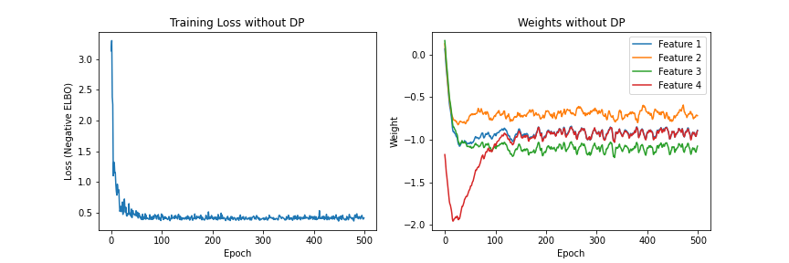
Test data에 대한 분류 정확도는 90.6%으로 도출되었다.
DPVI implementation
이번에는 앞선 DPVI 알고리즘을 살펴보도록 하겠다. 우선, DPVI에서는 각 반복(에포크)에서 주어진 sampling probability 로 랜덤 샘플 를 구성하고 이를 바탕으로 그래디언트를 계산하기 때문에, 랜덤 샘플링을 위한 코드가 필요하다. 주어진 데이터셋에서 샘플링을 수행하기 위해서는 Sampler 클래스를 이용하면 되는데, 다음과 같이 구성할 수 있다.
# Sampler
class RandomSampler(Sampler[int]):
    def __init__(self, data_source, sampling_prob):
        self.data_source = data_source
        self.sampling_prob = sampling_prob
        self.indices = [i for i in range(len(self.data_source)) if np.random.rand() < self.sampling_prob]

    def __len__(self):
        return len(self.indices)

    def __iter__(self):
        return iter(self.indices)

# Test the sampler
sampler = RandomSampler(train_dataset, 0.5)
dataloader = DataLoader(train_dataset, sampler=sampler)
len(dataloader) # 195 (random)
이를 기반으로 다음과 같이 DPVI 코드를 작성하였다.
# DPVI
torch.manual_seed(42)

loss_collection = dict()
beta_collection = dict()

for epsilon in [0.01, 0.1, 1.0, 10.0]:

    lr = 0.01
    n_epochs = 500
    losses = []
    betas = []
    sampling_prob = 0.05
    clipping_threshold = 5.0
    delta = 1e-3

    noise_multiplier = np.sqrt(2 * np.log(1.25 / delta)) / epsilon

    # Initialize the model

    model_dp = BayesianLogisticRegression(n_features=X.shape[1])
    optimizer = torch.optim.Adam(model_dp.parameters(), lr=lr)

    pbar = tqdm(range(n_epochs))

    # DPVI algorithm

    losses = []
    betas = []

    for epoch in pbar:
        beta_epoch = []
        loss_epoch = 0

        # Sample the minibatches (sampling_prob is the probability of including a sample in the minibatch)
        sampler = RandomSampler(train_dataset, sampling_prob)
        dataloader = DataLoader(train_dataset, sampler=sampler)

        # Initialize the accumulated gradients
        for p in model_dp.parameters():
            p.accumulated_grads = []

        for x, y in dataloader:
            optimizer.zero_grad()
            loss = model_dp.loss(x, y)
            loss.backward()
            loss_epoch += loss.item()

            for p in model_dp.parameters():
                per_sample_grad = p.grad.detach().clone()
                clip_grad_norm_(per_sample_grad, clipping_threshold) # in-place operation
                p.accumulated_grads.append(per_sample_grad)


        # Aggregate the gradients
        for p in model_dp.parameters():
            p.grad = torch.stack(p.accumulated_grads).sum(dim=0)
            p.grad += torch.randn_like(p.grad) * clipping_threshold * noise_multiplier

        optimizer.step()
        model_dp.zero_grad()

        betas.append(model_dp.mean.detach().numpy().copy())
        losses.append(loss_epoch / len(dataloader))

        pbar.set_description(f'epsilon={epsilon}')
        pbar.set_postfix({'loss': losses[-1]})

    losses = np.array(losses)
    betas = np.array(betas)

    loss_collection[epsilon] = losses
    beta_collection[epsilon] = betas
Privacy budget 을 달리하며 ELBO의 수렴을 비교한 플롯은 다음과 같다.
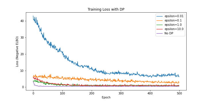
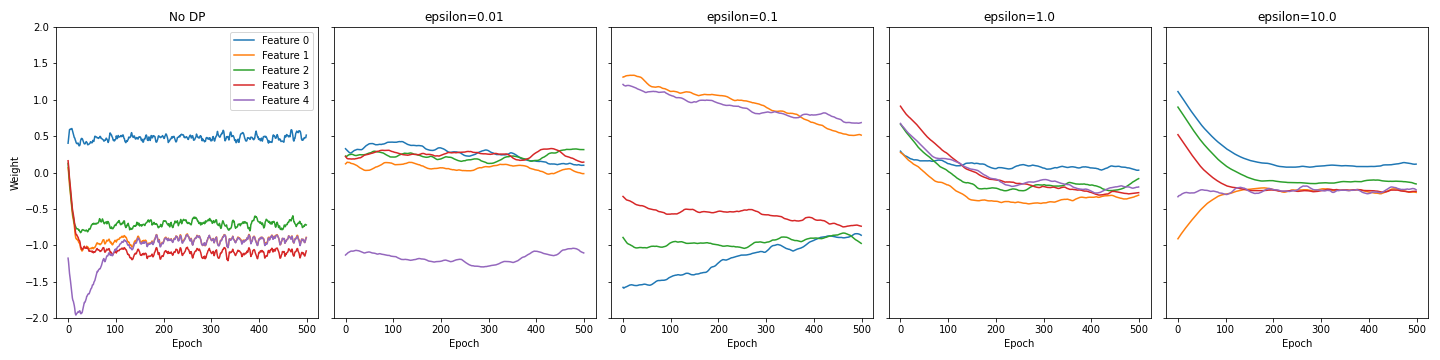
Privacy budget이 낮을수록 그래디언트에 더 많은 노이즈가 추가되기 때문에, 수렴 속도가 더 느린 것을 확인할 수 있다.
References
- Jälkö, J., Dikmen, O., & Honkela, A. (2017). Differentially Private Variational Inference for Non-conjugate Models (arXiv:1610.08749). arXiv. https://doi.org/10.48550/arXiv.1610.08749
- Wang, Y.-X., Fienberg, S., & Smola, A. (2015). Privacy for Free: Posterior Sampling and Stochastic Gradient Monte Carlo. Proceedings of the 32nd International Conference on Machine Learning, 2493–2502. https://proceedings.mlr.press/v37/wangg15.html
- M. Abadi et al., “Deep Learning with Differential Privacy,” in Proceedings of the 2016 ACM SIGSAC Conference on Computer and Communications Security, Oct. 2016, pp. 308–318. doi: 10.1145/2976749.2978318.
- A. Kucukelbir, D. Tran, R. Ranganath, A. Gelman, and D. M. Blei, “Automatic Differentiation Variational Inference,” Journal of Machine Learning Research, vol. 18, no. 14, pp. 1–45, 2017.