Intro

• Most existing work on DP-publication of location data focuses on single snapshot releases (Cormode et al., 2012)
• To release multiple snapshot, user-level privacy is required
• Two key aspects : Bound sensitivity and Add noise, with denoising step

Preliminaries

Problem Formulation

Goal

Release high-resolution density information of dataset $D$.

• Build a $M\times M\times T$ histogram $H$ over $D$, where $M,T$ is determined spatial and temporal resolution parameter.

Queries

1. Range count queries

   • Given the query range(max,min of lat, lon, time)
   • Return : the number of user location in $D$ that satisfy this range
   • Metric : relative error metric $\text{RE}(y,u) = \dfrac{\vert y-u\vert }{\max\lbrace u,\psi\rbrace }$
   • where $\psi$ is smoothing factor to avoid division by zero.

2. Nearest hotspot queries

   • Given query location $q$, density threshold $v$, spatio-temporal extent $SR$
   • Return : closest cell to $q$ within extents $SR$ that contains at least $v$ locations.
   • Metric : MAE between distance $H,\hat H$ for distance penalty. Regret (deviation of the reported density of the found hotspot from given $\hat H, v$) for hotspot density estimation error
   • $\text{Regret}(q)=0$ if the reported hotspot meets the density threshold $v$.

3. Forecasting queries

   • Given timeseries of spatial densities and forecasting horizon $h$
   • Return : The prediction of count of location reports for $h$ future timesteps.
   • Metric : symmetric mean absolute percentage errors
   $$\text{sMAPE} = \frac{1}{h}\sum_{t=1}^{h}\dfrac{\vert F_{t}-A_{t}\vert }{(A_{t}+F_{t})/2}$$

   where $A_{t}$ are the true counts from $H$ in the $h$ timesteps and $F_{t}$ are the $h$ predicted counts from a forecasting algorithm fitted to the historical data from $\hat H$.

Data

• Spatiotemporal data : have density patterns through both temporal and spatial axis. (e.g. weekday vs weekend pattern at commercial area) (Yang et al., n.d.)
• Distribution across users : power law distribution

VDR^{VAE-based Density Release}

• Differentially private release of spatiotemporal data

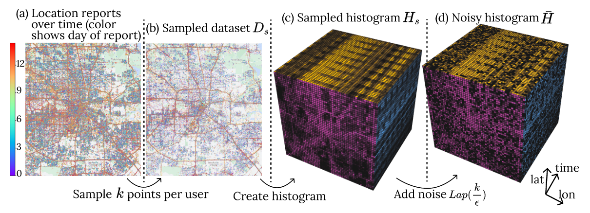
Data collection

• Goal is to create the $\epsilon$-DP histogram (Figure (d)).
• Laplace mechanism with sensitivity $\Delta=k_\text{max}$ i.e. the maximum number of points.

• Bound sensitivity by sampling a maximum of $k$ points per user.

Learned Denoising

1. Spatiotemporal dataset are similar to video(seq. of images)
2. Regularized representation learning > learns denoised representation without overfitting
3. Multi-resolution learning can capture spatio-temporal patterns at different resolution

Design Principles

• Denoising with regularized representation learning

  : Derive a denoised histogram $\hat H$ from VAE that minimizes reconstruction loss $\Vert \hat H - \bar H\Vert$ . By setting the dimensionality of representation lower than $\bar H$, the representation will capture the patterns in $\bar H$.

• Multi-resolution Learning

  : Prepare the training set with $r$ different resolution scales. Expect to improve denoising accuracy via MRL.

Algorithm

Model

• Given a noisy ST histogram $\bar H= \lbrace \bar H_i\rbrace _{i=1}^{T}$ where $\bar H_i$ is a spatial histogram at $i$-th timestamp.
• For regularized representation learning, use Convolutional VAE.
• $\text{encoder}(.;\theta_{e})$ : 2D histogram (any resolution) > representation $\in \mathbb{R}^{n\times l}$
• $\text{decoder}(.;\theta_{d})$ : representation > 2D histogram
• Inference : Given $\bar H_i$, obtain $\hat H$ (3D histogram).

VQ-VAE (Razavi et al., 2019)

• $\Gamma=\lbrace e_{1},\ldots,e_{B}\rbrace$ : codebook of $B$ different discrete encodings
• For training set $\bar T$, $\text{encoder}(\bar T:\theta_{e})$ produces a set of representations $z$.
• $L_{G}(z) = d(z,\Gamma)$ : regulariaztion loss. distance between representation and codebook
• $L_{C}(\hat T) = \sum_{i=1}^{\vert \bar T\vert }\Vert \bar T_{i}-\hat T_{i}\Vert^{2}$ : reconstruction loss
• Optimization becomes:

• Parameters
  • $B$ : variability of the encoding space (representation power)
  • $\alpha$ : How much the encoder is forced to adhere to the codebook.
  • Experiment : $\alpha=1, \beta=128$

Statistical Analysis

Let $X_{i}^{c}$ be the Bernoulli random variable indicates whether $i$th point falls in a cell $c$. Suppose the $i$th point is sampled from $\text{Uniform}(D)$. Let $\mathrm{E}X_{i}^{c}=\mu_{c}$. The estimator is given by

Then, the bias and variance can be calculated as follows.

where $N=\vert D\vert$ is the total number of data points and $n=\vert D_{s}\vert$ is the total number of sampled data. Thus, the MSE is given by

By differentiating w.r.t. $\gamma$, we obtain

minimizes $\sum_{c}\text{MSE}(\theta_{c})$ where $C=\sum_{c=1}^{m}\mu_{c}^{2}$ is a data-dependent constant.

Theorem

The following VDR algorithm is $\epsilon$-DP.

References

• Ahuja, R., Zeighami, S., Ghinita, G., & Shahabi, C. (2023). A Neural Approach to Spatio-Temporal Data Release with User-Level Differential Privacy. Proceedings of the ACM on Management of Data, 1(1), 1–25. https://doi.org/10.1145/3588701
• Razavi, A., Oord, A. van den, & Vinyals, O. (2019). Generating Diverse High-Fidelity Images with VQ-VAE-2 (arXiv:1906.00446). arXiv. https://doi.org/10.48550/arXiv.1906.00446
• Cormode, G., Procopiuc, C., Srivastava, D., Shen, E., & Yu, T. (2012). Differentially Private Spatial Decompositions. 2012 IEEE 28th International Conference on Data Engineering, 20–31. https://doi.org/10.1109/ICDE.2012.16