Gaussian Process Classification
Classification Problem
분류 문제의 두 가지 관점
베이지안 관점에서 분류(Classification) 문제를 정의하는 과정을 생각해보면, 설명변수 $\mathbf{x}$와 반응변수(class) $y$의 결합확률분포 $p(y,\mathbf{x})$를 접근하는 방식에 두 가지 방법이 있음을 고려할 수 있다.
\[p(y,\mathbf{x}) = p(y)p(\mathbf{x}\vert y) = p(\mathbf{x})p(y\vert \mathbf{x})\]두 번째 항과 세 번째 항 모두 조건부 분포를 정의하는 것에 의해 표현되며, 이때 두 접근 방법을 각각 generative approach, discriminative approach 라고 한다.
Generative approach
Generative approach에서는 class-conditional distribution $p(\mathbf{x}\vert y)$ 를 모델링하고, 각 class($C_{1},\ldots ,C_{C}$)에 대한 사전분포를 설정하여 다음과 같이 사후확률분포를 구한다.
\[p(y\vert \mathbf{x}) = \frac{p(y)p(\mathbf{x}\vert y)}{\sum_{c=1}^{C}p(C_{c})p(\mathbf{x}\vert C_{c})}\]Discriminative approach
반면, discriminative approach의 경우에는 response function $\sigma:\mathbb{R}\to [0,1]$ 을 사용하여 설명변수가 주어질 때 각 클래스에 속할 확률을 모델링한다. 아래는 이러한 접근법을 사용한 예시로 선형 로지스틱 회귀모형을 나타낸다.
\[p(C_{1}\vert \mathbf{x})=\lambda(\mathbf{x^{T}w})\qquad \lambda(z)=\frac{1}{1+\exp(-z)}\]이번 포스팅에서 다룰 Gaussian Process를 이용한 분류 모형은 discriminative approach에 기반한 것이다.
Linear Classification
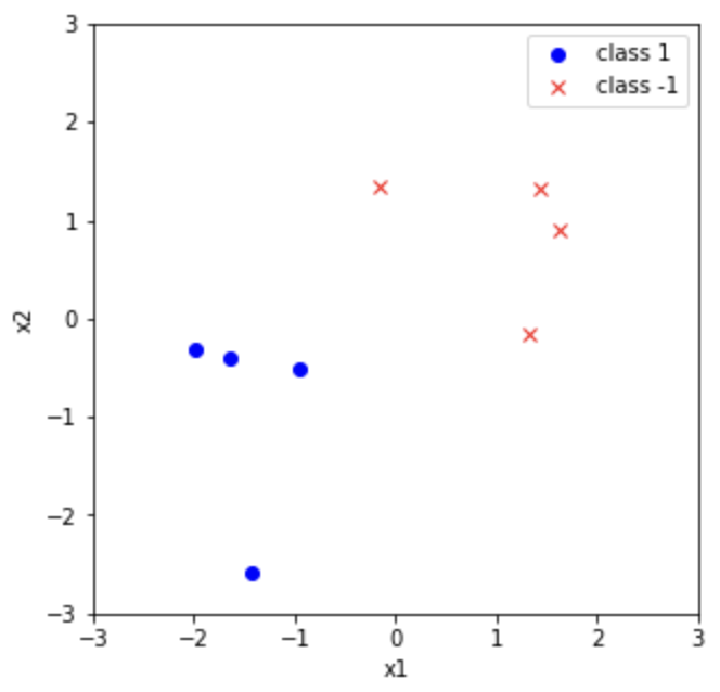
Gaussian Process Classifier를 다루기에 앞서, 우선 간단한 선형분류기를 살펴보도록 하자. 반응변수가 두 가지 클래스($+1,-1$)를 갖고 다음과 같이 가능도함수가 주어진다고 하자.
\[p(y=+1\vert \mathbf{x,w})=\sigma(\mathbf{x}^T\mathbf{w})\]또한, 주어진 분류 문제에서 데이터셋이 \(\mathcal{D}=\lbrace (\mathbf{x}_{i}, y_{i})\vert i=1,\ldots,n\rbrace\) 으로 주어지고, parameter $\mathbf{w}$ 에 대한 가우시안 사전분포($\mathbf{w}\sim N(0,\Sigma_{p})$)를 정해주면 다음과 같은 로그사후확률분포를 구할 수 있다.
\[\log p(\mathbf{w}\vert X,Y)=- \frac{1}{2}\mathbf{w}^{T} \Sigma_{p}^{-1}\mathbf{w} + \sum _{i=1}^{n}\log \sigma(y_{i},f_{i})\]다만, 식으로부터 알 수 있다시피 회귀모형과는 다르게 MAP estimator의 closed form을 구할 수 없다. 대신 특정 response function(로지스틱, 정규분포 cdf)등을 사용했을 때 위 로그사후분포의 형태가 concave function이 되고, 이를 이용하면 Newton-Raphson 등을 이용해 추정량을 구할 수 있다.
Example
- $\mathbf{w}\in \mathbb{R}^{2}, \mathbf{x}_{i}\in\mathbb{R}^{2}, i=1,\ldots,8$
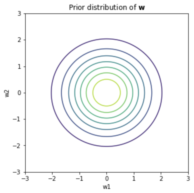
- Prior Distribution $\mathbf{w} \sim N(0, I_{2})$
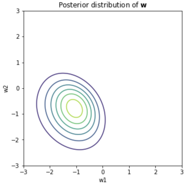
- Posterior Distribution $p(\mathbf{w}\vert \mathbf{x})$
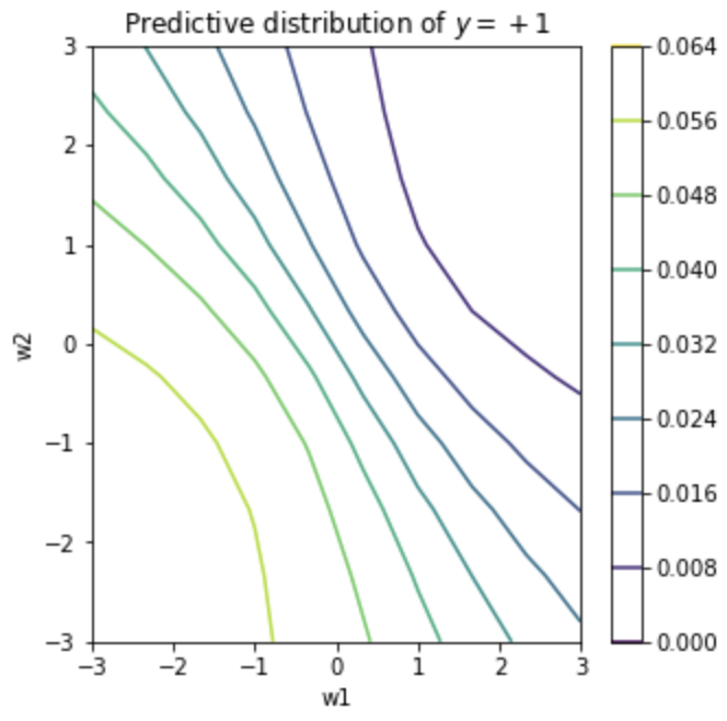
- Predictive Distribution
Gaussian Process Classification
분류 문제에서 Gaussian Process를 사용하는 것은 단지 latent function이라 하는 함수 $f(\mathbf{x})$ 에 대해 gaussian process 사전분포를 설정하는 것이다. 다만, 앞서 설명한 discriminative approach에서 도출해야 하는 것은 각 데이터들에 대한 클래스별 확률값(0과 1 사이)이므로, 로지스틱 함수와 같은 sigmoid를 거친 $\pi(\mathbf{x})=\sigma(f(\mathbf{x}))$ 를 이용하게 된다. 계산의 편의를 위해 관측모형이 noise-free, 즉 $y=f(\mathbf{x})$ 로 noise term($\epsilon$) 없이 직접 표현된다고 가정하자.
Inference
추론 과정은 우선 test data $x_{\ast}$에 대한 latent variable $f_{\ast}$ 의 확률분포를 계산하는 것으로부터 시작된다.
\[p(f_{\ast}\vert X,y,x_{\ast})= \int p(f_{\ast}\vert X,x_{\ast},\mathbf{f})p(\mathbf{f}\vert X,y)d\mathbf{f}\]여기서 input data에 대한 latent variable $\mathbf{f}$의 posterior distribution은 다음과 같다.
\[p(\mathbf{f}\vert X,y) = \frac{p(y\vert \mathbf{f})p(\mathbf{f}\vert X)}{p(y\vert X)}\]다음으로, 이를 이용하여 test data에 대한 예측 확률을 다음과 같이 계산할 수 있다.
\[\bar\pi_{\ast} := p(y_{\ast}=+1\vert X,y,x_{\ast}) = \int \sigma(f_{\ast})p(f_{\ast}\vert X,y,x_{\ast})df_{\ast}\]Gaussian Process Regression의 경우와 다른 것은, posterior distribution
\[p(\mathbf{f\vert X,y})\]가 gaussian distribution이 아니므로, 가능도함수를 직접 계산하는 방식으로 추론 및 예측하는 것은 어렵다. 이를 위해 non-Gaussian joint posterior를 근사하기 위한 Laplace approximation, Expectation propagation 혹은 MCMC approximation 등이 사용된다.
References
- Gaussian Process for Machine Learning
- Code on Github
Leave a comment