Laplace Approximation Binary GP Classifier
바로 이전 글에서 Gaussian Process classifier는 사후확률분포가 정규분포형태가 아니고, 이로 인해 직접 계산이 어렵다는 점을 살펴보았다. Laplace Approximation은 사후확률분포 $p(\mathbf{f}\vert X,y)$ 를 정규분포 형태로 근사할 수 있는 테크닉이다.
Laplace Approximation
베이즈 규칙에 의해 latent variable $\mathbf{f}$ 의 사후확률분포는 다음과 같이 주어진다.
\[p(\mathbf{f}\vert X,y)\propto p(y\vert \mathbf{f})p(\mathbf{f}\vert X)\]로그를 취하고 Gaussian process prior distribution을 적용하면,
\[\begin{aligned} \Psi(\mathbf{f}) &:= \log p(y\vert \mathbf{f})+\log p(\mathbf{f}\vert X)\\ &= \log p(y\vert \mathbf{f}) - \frac{1}{2}\mathbf{f}^{T}K^{-1}\mathbf{f}- \frac{1}{2}\log\vert K\vert - \frac{n}{2}\log 2\pi \end{aligned}\]가 된다. 위 식을 $\mathbf{f}$ 에 대해 미분하면, 다음과 같이 그래디언트 및 헤시안 행렬을 얻을 수 있다.
\[\begin{aligned} \nabla\Psi(\mathbf{f}) &= \nabla\log p(y\vert \mathbf{f})-K^{-1}\mathbf{f}\\ \nabla\nabla\Psi(\mathbf{f}) &= -W-K^{-1} \end{aligned}\]또한, 사후확률을 최대로 하는 latent variable을 찾으면
\[\hat{\mathbf{f}} = K(\nabla\log p(y\vert \mathbf{\hat f}))\]가 되고, closed form이 존재하지 않으므로 다음과 같이 Newton algorithm을 이용해 구할 수 있다.
\[\begin{aligned} \mathbf{f}^{\mathrm{new}}&= \mathbf{f}-(\nabla^2\Psi)^{-1}\nabla\Psi\\ &= (K^{-1}+W)^{-1}(W\mathbf{f}+\nabla\log p(y\vert \mathbf{f})) \end{aligned}\]이를 통해 MAP estimator $\mathbf{\hat f}$ 를 찾으면 이를 이용해 다음과 같은 사후분포의 Laplace approximation을 얻게 된다.
\[q(\mathbf{f}\vert X,y) \sim N(\mathbf{\hat f},(K^{-1}+W)^{-1})\]Prediction
Test data $x_{\ast}$에 대한 predictive distribution을 구하는 과정에서 앞서 구한 Laplace approximation을 이용하면 다음과 같다. 우선 test data에 대한 latent mean은
\[\begin{aligned} \mathrm{E}_{q}[f_{\ast}\vert X,Y,x_{\ast}] &= \int \mathrm{E}[f_{\ast}\vert \mathbf{f},X,x_{\ast}]q(\mathbf{f}\vert X,y)d\mathbf{f} \\ &= \int \mathbf{k}(x_{\ast})^{T}K^{-1}\mathbf{f}q(\mathbf{f}\vert X,y )d\mathbf{f}\\ &= \mathbf{k}(x_{\ast})^{T}K^{-1}\mathrm{E}_{q}[\mathbf{f}\vert X,y]\\ &= \mathbf{k}(x_{\ast})^{T}K^{-1}\mathbf{\hat f} \\ &= \mathbf{k}(x_{\ast})^{T}\nabla\log p(y\vert \mathbf{\hat f}) \end{aligned}\]으로 주어지고, 이를 이용하면 실제 prediction $\pi_{\ast}$ 에 대한 MAP estimator는 다음과 같이 구할 수 있다.
\[\begin{aligned} \bar\pi_{\ast}&= \mathrm{E_{q}[\pi_{\ast}\vert X,Y,x_{\ast}}]\\ &= \int \sigma(f_{\ast})q(f_{\ast}\vert X,Y,x_{\ast})df_{\ast} \end{aligned}\]Example
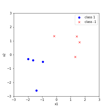
이전 Linear Classification Model에서 다루었던 데이터를 바탕으로 예측 확률분포를 구하는 과정을 알고리즘으로 살펴보도록 하자. 우선 데이터는 다음과 같이 각 클래스별로 4개씩 주어졌다고 가정하자.
Kernel function은 Gaussian RBF
\[k(\mathbf{x_{1},x_{2}}) = \exp(-\Vert\mathbf{x}_{1}-\mathbf{x}_{2}\Vert^{2})\]을 사용했으며, 우선 이를 이용해 Covariance Matrix $K$와 로그가능도 $\log p(y\vert \mathbf{f})$ 를 구한다.
# covariance matrix

K = np.array([[kernel(X[i], X[j]) for j in range(2*N)] for i in range(2*N)])

# logistic Likelihood

def loglik(y, f):
	return np.sum(np.log(1 + np.exp(-y*f)))
Laplace Approximation의 알고리즘은 다음과 같다.
# Laplace approximation
from scipy.integrate import quad

def laplace_approximation(y, K, X, x_new=None, max_iter=100):
    N = len(y)
    f = np.zeros(N)
    for i in range(max_iter):
        pi = np.exp(f) / (1 + np.exp(f))
        W = np.diag(pi * (1 - pi))
        W_sqrt = np.sqrt(W)
        L = np.linalg.cholesky(np.eye(N) + W_sqrt.dot(K).dot(W_sqrt)) # Cholesky decomposition
        t = (y + np.ones(N)) / 2 - pi
        b = W.dot(f) + t
        a = b - W_sqrt.dot(np.linalg.solve(L.T, np.linalg.solve(L, W_sqrt.dot(K).dot(b))))
        f = K.dot(a)

    pi = np.exp(f) / (1 + np.exp(f))
    W = np.diag(pi * (1 - pi))
    W_sqrt = np.sqrt(W)
    L = np.linalg.cholesky(np.eye(N) + W_sqrt.dot(K).dot(W_sqrt))
    t = (y + np.ones(N)) / 2 - pi
    b = W.dot(f) + t
    a = b - W_sqrt.dot(np.linalg.solve(L.T, np.linalg.solve(L, W_sqrt.dot(K).dot(b))))

    # approximate marginal log likelihood
    def q(y, X):
        return -0.5 * a.T.dot(f) + loglik(y, f) - np.sum(np.log(np.diag(L)))

    if x_new is None:
        return f, q, pi

    else:
        # predictive mean
        k_new = np.array([kernel(x_new, X[i]) for i in range(len(X))])
        f_new = k_new.dot(t)
        # predictive variance
        v = np.linalg.solve(L, W_sqrt.dot(k_new))
        v_new = np.array(kernel(x_new, x_new)) - v.dot(v)
        # predictive class probability
        def integrand(z):
            return 1 / (1 + np.exp(-z)) * multivariate_normal(mean = f_new, cov = v_new).pdf(z)
        pi_new = quad(integrand, -100, 100)[0]

        return f_new, pi_new
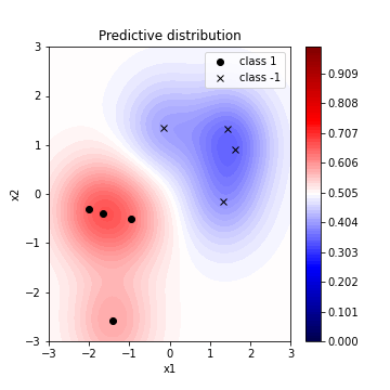
이를 바탕으로 Predictive distribution의 contour plot을 다음과 같이 그릴 수 있다.
References
- Gaussian Process for Machine Learning
- Code on Github
Leave a comment