Archive
PyMC 라이브러리를 활용한 베이지안 분석
PyMC and Bayesian 이번 글에서는 Python에서 MCMC 기반의 베이지안 분석을 할 수 있도록 고안된 PyMC 라이브러리를 소개해보도록 하겠습니다. PyMC에서는 비교적 간단한 MCMC부터, Bayesian neural network BNN 까지 폭넓은 분석을 진행할 수 있습니다. 여기서는 선형회귀모형과 로지스틱 회귀모형, 그리고 BNN을 활용한 분류를 다루어보도록 하겠습...
PyMC and Bayesian
이번 글에서는 Python에서 MCMC 기반의 베이지안 분석을 할 수 있도록 고안된 PyMC 라이브러리를 소개해보도록 하겠습니다. PyMC에서는 비교적 간단한 MCMC부터, Bayesian neural networkBNN까지 폭넓은 분석을 진행할 수 있습니다. 여기서는 선형회귀모형과 로지스틱 회귀모형, 그리고 BNN을 활용한 분류를 다루어보도록 하겠습니다.
MCMC
MCMC에 대한 이론적인 설명은 관련 글을 참고바랍니다. pymc에서 MCMC는 pm.sample 함수를 이용해 수행할 수 있습니다. 예시로 다음과 같은 상황을 가정합니다.
즉, 정규분포의 모수 에 대해 Cauchy 사전분포를 가정합니다. 여기서는 으로 하였으며, 관측 데이터 observation은 다음과 같이 평균이 3인 정규분포에서 생성하였습니다.
np.random.seed(123)

n = 100
observation = norm.rvs(3, 1, n)
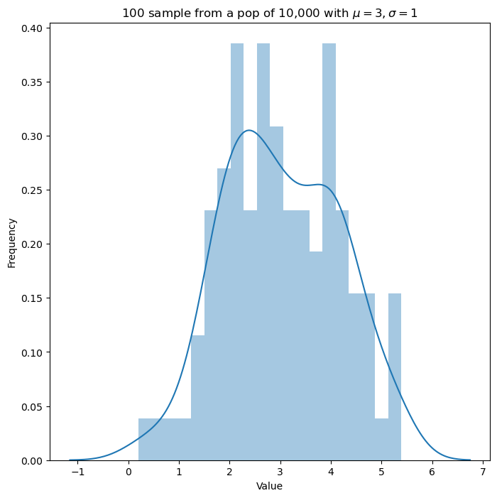
대략적인 분포는 다음과 같습니다.
fig, ax = plt.subplots(1,1, figsize=(8,8))
sns.distplot(observation, ax=ax, kde=True, bins=20)
plt.xlabel("Value")
plt.ylabel("Frequency")
plt.title("100 sample from a pop of 10,000 with $\mu=3, \sigma=1$")
plt.show()
이 경우 다음과 같이 사후분포와 제안분포를 계산하여 Metropolis-Hasting 알고리즘을 수행할 수 있습니다.
pymc에서는, pm.Metropolis()를 이용해 MH 알고리즘을 수행할 수 있습니다. 코드는 다음과 같습니다.
# MH algorithm

ex2 = pm.Model()

with ex2:
    # Cauchy 사전분포
    mu = pm.Cauchy('mu', 0, 1)
    # 관측값의 분포(가능도)
    y = pm.Normal('y', mu=mu, sigma=1, observed=observation) # observed 값에 관측값 벡터를 넣어준다.
    # Metropolis-Hastings 알고리즘
    trace = pm.sample(10000, tune=1000, step=pm.Metropolis())
일반적으로 pymc 라이브러리를 활용하는 분석과정은 위 코드와 같이 pm.Model() 클래스를 지정해주고, with 구문을 이용해 내부에 사전분포, 가능도 등의 변수를 지정해주게 됩니다.
pm.Cauchy, pm.Normal 등의 함수는 확률변수를 지정해주는 클래스입니다. 이를 바탕으로 위 코드와 같이 가능도를 구성할 수 있으며, pm.sample 함수에 샘플링 알고리즘인 pm.Metropolis를 지정하여 MCMC를 수행할 수 있습니다.
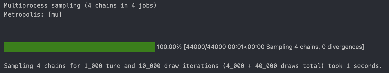
코드를 실행하면 아래와 같이 반복적으로 샘플링이 이루어지는 과정을 확인할 수 있습니다(Jupyter 기준). 여기서 chain은 총 4개가 사용되었는데, chain이란 MCMC를 수행하는 개별 Markov chain을 의미합니다. 즉, 4개의 Markov chain을 활용하여 각각에 대해 독립적인 샘플링을 수행한 것을 의미합니다.
또한, tune=1000 옵션은 MCMC의 burn-in 문제를 해결하기 위해 샘플로 취급하지 않는 초반의 반복 과정을 의미합니다. 여기서는 초기 1000번의 반복 횟수를 burn-in period로 처리한다는 것을 의미하고, 이후 과정에 대해 10000번의 샘플을 (각 chain마다) 추출하게 됩니다.
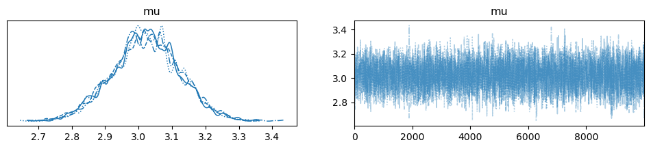
이 과정에서 trace에 arviz 객체가 저장되는데, 이는 각 chain, step에서의 샘플 값을 저장한 다차원 배열입니다. MCMC로 얻은 사후분포를 확인하기 위해 다음과 같이 trace 객체에 대한 plot을 그릴 수 있습니다.
# Trace plot
pm.plot_trace(trace)
plt.show()
왼쪽 plot의 서로 다른 네 그래프는 각각 개별 Markov chain의 사후분포에 대응됩니다. 또한, 다음 코드를 실행시켜 MAPmaximum a posterior 추정량을 구할 수 있습니다.
# MAP estimate
pm.find_MAP(model=ex2)
# {'mu': array(3.02114274)}
데이터가 생성된 평균 3.0에 근접하게 도출된 것을 확인할 수 있습니다.
Linear Regression
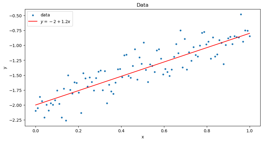
이번에는 다음과 같은 회귀직선에서의 데이터를 고려해봅시다.
# Data Generate

n = 100
true_beta_0 = -2.0
true_beta_1 = 1.2

x = np.linspace(0,1,n)
y = true_beta_0 + true_beta_1 * x + np.random.normal(0, 0.2, n)

plt.figure(figsize=(10, 5))
plt.scatter(x, y, label='data', s=10)
plt.plot(x, true_beta_0 + true_beta_1 * x, c='r', label='$y = -2 + 1.2x$')
plt.legend()
plt.xlabel("x")
plt.ylabel("y")
plt.title("Data")
plt.show()
베이지안 추론을 적용하기 위해, 다음과 같이 모델을 만들고 MH 알고리즘을 적용할 수 있습니다. 회귀계수 에 각각 정규사전분포를 설정하였으며, 오차항의 분포에는 사전분포 없이 인 정규분포를 적용하였습니다.
# Bayesian Linear Regression

ex_linreg = pm.Model()

with ex_linreg:
    # 사전분포
    beta_0 = pm.Normal('beta_0', mu=0, sigma=10)
    beta_1 = pm.Normal('beta_1', mu=0, sigma=10)

    # 관측값의 분포(가능도)
    y = pm.Normal('y', mu=beta_0 + beta_1 * x, sigma=0.2, observed=y)

    # MCMC 알고리즘
    trace = pm.sample(10000, tune=1000, step=pm.Metropolis())
trace 객체의 trace plot을 그려보면 다음과 같습니다.
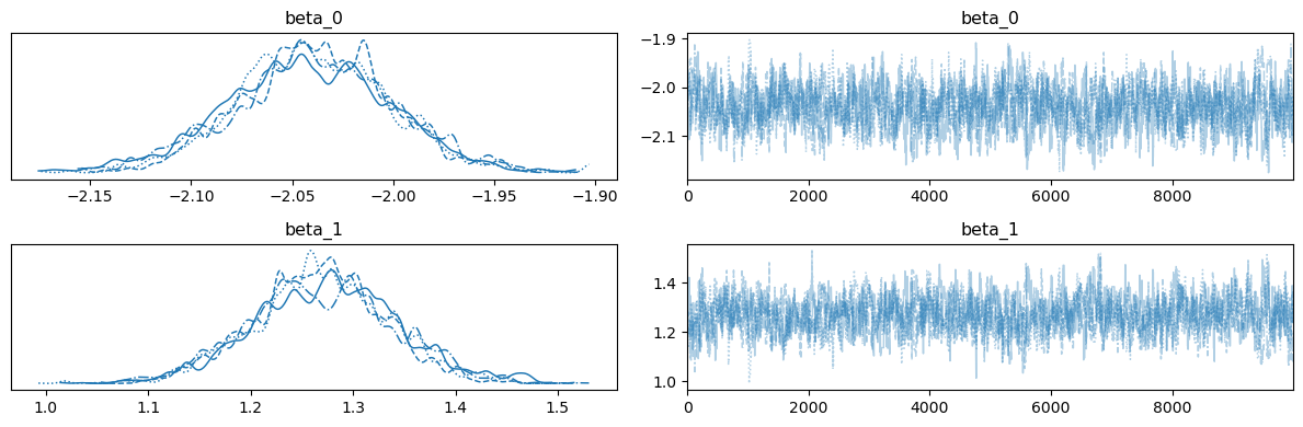
MAP 추정량을 구하면, 실제 샘플이 생성된 회귀계수에 거의 일치하는 것을 알 수 있습니다.
# MAP estimate

pm.find_MAP(model=ex_linreg)
# {'beta_0': array(-2.03997915), 'beta_1': array(1.26967773)}
Bayesian Logistic Regression
로지스틱 회귀도 동일한 알고리즘으로 진행할 수 있습니다. 가능도함수로 정규분포 대신, 시그모이드 함수와 베르누이 확률변수를 이용하면 됩니다. 여기서는 iris 데이터셋을 이용하여 두 가지 클래스(setosa, versicolor)와 두 가지 변수(sepal_length, sepal_width)에 대한 모델을 만들었습니다.
import seaborn as sns
from sklearn.preprocessing import LabelEncoder, StandardScaler

iris = sns.load_dataset('iris')
iris = iris.loc[iris.species.isin(['setosa','versicolor']), ['sepal_length', 'sepal_width', 'species']]

X = iris[iris.columns.drop('species')].to_numpy()

X = StandardScaler().fit_transform(X)
y = LabelEncoder().fit_transform(iris['species'])

print(X.shape, y.shape) # (100, 2) (100,)
산점도로 데이터를 표현하면 다음과 같습니다.
# Plot the data

fig, ax = plt.subplots(1, 1, figsize=(7, 7))

sns.scatterplot(x=X[:,0], y=X[:,1], hue=y, ax=ax)
ax.legend(loc='upper right')
plt.show()
마찬가지로, pymc의 Model 모듈을 활용하여 다음과 같이 GLM을 구성할 수 있습니다.
- Prior : 각 회귀계수에 대해() 정규사전분포 부여
- Likelihood : 가능도함수(여기서는 이진 분류 문제이므로 베르누이 분포)
pm.invlogit 함수를 활용하여 로지스틱 함수 를 사용할 수 있습니다.
with pm.Model() as model:
    # Priors
    intercept = pm.Normal('Intercept', 0, sigma=100)
    x1_coef = pm.Normal('sepal_length', 0, sigma=100)
    x2_coef = pm.Normal('sepal_width', 0, sigma=100)

    # Likelihood
    likelihood = pm.invlogit(intercept + x1_coef*X[:,0] + x2_coef*X[:,1])

    # Bernoulli random variable
    y_obs = pm.Bernoulli('y', p=likelihood, observed=y)

    trace = pm.sample(3000, tune=1000, chains=4)
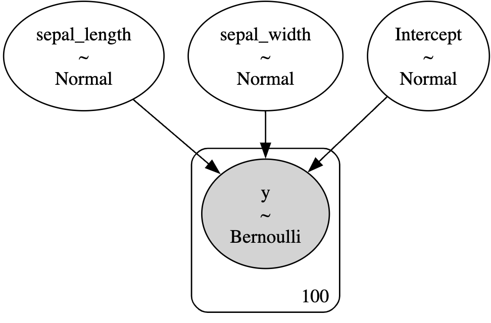
pm.model_to_graphviz(model) 코드를 실행시키면, 구성한 모델이 어떠한 형태로 이루어져있는지 그래피컬 모델 형태로 확인할 수 있습니다. 아래 그림과 같이, 종속변수 회귀계수의 사전분포와, 반응변수의 가능도가 어떠한 확률분포를 갖는지 확인할 수 있습니다.
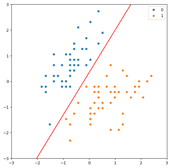
아래는 MAP 추정량을 활용한 결정경계를 그리기 위한 코드입니다.
# MAP estimate

with model:
    map_estimate = pm.find_MAP()

print(map_estimate)

# Plot the decision boundary

x1 = np.linspace(-3.0, 3.0, 100)
x2 = np.linspace(-3.0, 3.0, 100)

X1, X2 = np.meshgrid(x1, x2)

X_new = np.vstack([X1.ravel(), X2.ravel()]).T

# MAP estimate

y_probs = 1 / (1 + np.exp(-(map_estimate['Intercept'] + map_estimate['sepal_length'] * X_new[:,0] + map_estimate['sepal_width'] * X_new[:,1])))
y_probs = y_probs.reshape(100, 100)

# Plot

fig, ax = plt.subplots(1, 1, figsize=(7, 7))

sns.scatterplot(x=X[:,0], y=X[:,1], hue=y, ax=ax)
ax.legend(loc='upper right')
ax.contour(X1, X2, y_probs, levels=[0.5], colors='r')

plt.show()
Bayesian Neural Network
일반적인 심층신경망 모형은 지정된 차원의 parameter matrix 를 주어진 데이터로부터 학습합니다. 이때, 여타 베이지안 이론들과 마찬가지로 parameter 를 직접 구하기보다는, 의 사전분포를 설정하여 사후분포를 구하는 방법을 고려할 수 있습니다. 이러한 접근 방식을 사용하는 신경망 구조를 Bayesian neural network라고 하며, 앞선 pymc 모델들과 비슷한 방법으로 모델을 만들 수 있습니다. 이론에 대한 자세한 내용은, 추후 별도의 포스트로 다루도록 하겠습니다.
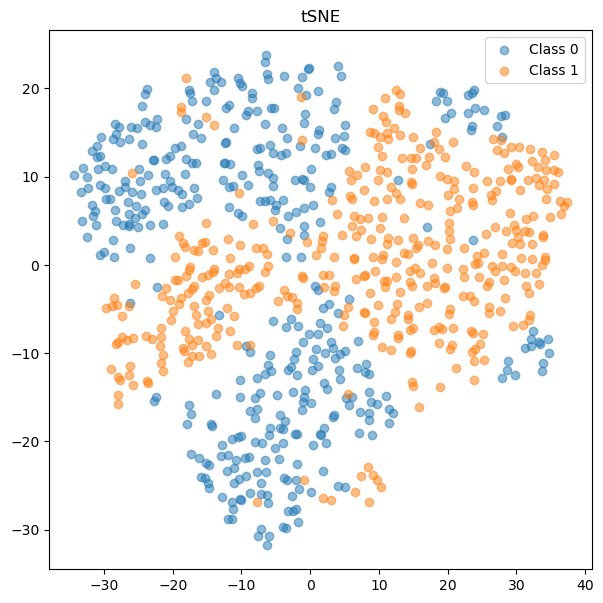
여기서는 분류 문제를 다루며, 사용할 데이터셋은 scikit-learn의 make_classification 모듈을 활용하여 toy data를 만들었습니다. 데이터셋의 생성 코드와 tSNE 플롯은 다음과 같습니다.
from sklearn.datasets import make_classification
from sklearn.model_selection import train_test_split
from sklearn.manifold import TSNE

X, y = make_classification(n_samples=1000, n_features=20, n_informative=10, n_classes=2, random_state=0, n_clusters_per_class=1)

X_train, X_test, y_train, y_test = train_test_split(X, y, test_size=0.2, random_state=0)

# plot tSNE

tsne = TSNE(n_components=2, random_state=0)
X_train_tsne = tsne.fit_transform(X_train)

plt.figure(figsize=(7, 7))
plt.scatter(X_train_tsne[y_train==0, 0], X_train_tsne[y_train==0, 1], label='Class 0', alpha=0.5)
plt.scatter(X_train_tsne[y_train==1, 0], X_train_tsne[y_train==1, 1], label='Class 1', alpha=0.5)
plt.title('tSNE')
plt.legend()
plt.show()
BNN을 생성하는 함수 construct_nn을 다음과 같이 정의하였습니다.
def construct_nn(ann_input, ann_output):
    n_hidden = 32

    # Initialize random weights between each layer
    init_1 = np.random.normal(size=(X_train.shape[1], n_hidden))
    init_2 = np.random.normal(size=(n_hidden, n_hidden))
    init_out = np.random.normal(size=n_hidden)

    coords = {
        "W1": np.arange(n_hidden),
        "W2": np.arange(n_hidden),
        "features": np.arange(X_train.shape[1]),
        # "obs_id": np.arange(X_train.shape[0]),
    }
    with pm.Model(coords=coords) as bnn:
        ann_input = pm.Data("ann_input", X_train, mutable=True, dims=("obs_id", "features"))
        ann_output = pm.Data("ann_output", y_train, mutable=True, dims="obs_id")

        # Weights from input to hidden layer
        weights_in_1 = pm.Laplace(
            "w_in_1", mu=0, b=1, initval=init_1, dims=("features", "W1")
        )

        # Weights from 1st to 2nd layer
        weights_1_2 = pm.Laplace(
            "w_1_2", mu=0, b=1, initval=init_2, dims=("W1", "W2")
        )

        # Weights from hidden layer to output
        weights_2_out = pm.Normal("w_2_out", 0, sigma=1, initval=init_out, dims="W2")

        # Build neural-network using tanh activation function
        act_1 = pm.math.maximum(0,pm.math.dot(ann_input, weights_in_1))
        act_2 = pm.math.maximum(0, pm.math.dot(act_1, weights_1_2))
        act_out = pm.math.sigmoid(pm.math.dot(act_2, weights_2_out))

        # Binary classification -> Bernoulli likelihood
        out = pm.Bernoulli(
            "out",
            act_out,
            observed=ann_output,
            total_size=y_train.shape[0],  # IMPORTANT for minibatches
            dims="obs_id",
        )
    return bnn
BNN에서 가중치 행렬의 sparsity를 부여하는 방법으로 Laplace 사전분포를 주는 방법이 있습니다. 여기서는 첫번째 레이어의 가중치와 두번째 레이어의 가중치 행렬에 각각 Laplace 사전분포 을 부여했습니다. 활성함수로는 ReLU 함수를 사용하기 위해, pm.math.maximum 함수를 이용하였고, 마지막 output layer에서는 시그모이드 활성함수를 사용하였습니다.
pm.ADVI 클래스를 이용하면, mean-field approximation을 가정한 자동미분Automatic Differentiation 기반의 변분추론을 수행할 수 있습니다.
BNN = construct_nn(X_train, y_train)

with BNN:
    advi = pm.ADVI()
    approx = pm.fit(30000, method=advi)
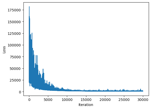
ELBO를 최대화하는 방향으로 손실함수를 설정하게 되며, 학습 과정에서의 손실함수 변화를 plot으로 나타내면 다음과 같이 학습 과정을 확인할 수 있습니다.
# Plot ELBO
plt.plot(approx.hist)
plt.xlabel("Iteration")
plt.ylabel("Loss")
plt.show()
이제, test data에 대해 예측을 진행해보고 정확도를 측정해보았습니다. BNN에서의 예측은, 각 테스트 데이터에 대해 여러 사후분포 샘플과(여기서는 1000개) 여러 chain(여기서는 4개)에 대한 샘플을 이용하여, 이들의 평균을 예측값으로 사용합니다.
with BNN:
    trace = approx.sample(1000)

# Test set

with BNN:
    pm.set_data({"ann_input": X_test, "ann_output": y_test})
    ppc = pm.sample_posterior_predictive(trace)
ppc객체에는 개별 사후분포 샘플, chain 별 예측값들이 저장되어있기 때문에, 다음과 같이 평균을 구하고 np.where 함수를 이용하여 예측확률이 0.5 이상인 개체를 class 1로 분류하였습니다.
# Accuracy

from sklearn.metrics import accuracy_score

accuracy_score(y_test, np.where(ppc.posterior_predictive['out'].mean(('chain', 'draw')) > 0.5, 1, 0))

# 0.99
로지스틱 회귀모형과 비교하면, 조금의 성능 향상이 있음을 확인할 수 있습니다.
from sklearn.linear_model import LogisticRegression

clf = LogisticRegression(random_state=0).fit(X_train, y_train)
y_pred = clf.predict(X_test)

accuracy_score(y_test, y_pred)

# 0.96
References
- PyMC official document
- Murphy, K. P. (2023). Probabilistic machine learning: Advanced topics. The MIT Press.