MM algorithm
MM algorithm은 EM algorithm의 일반화된 버전으로 이해하면 되는데, MM은 maximization 관점에서 minorize-maximize를 나타낸다. MM algorithm은 최대화하고자 하는 목적함수 $l(\theta)$ 에 대한 lower bound function(surrogate function) $Q(\theta,\theta^{t})$ 를 찾고 이를 maximize하는 $\theta^{t+1}$을 찾아 updating하는 방식으로 이루어진다. 이 메커니즘은 다음과 같은 monotonic increasing property를 보장한다.
\[l(\theta^{t+1})\geq Q(\theta^{t+1},\theta^{t})\geq Q(\theta^{t},\theta^{t})=l(\theta^t)\]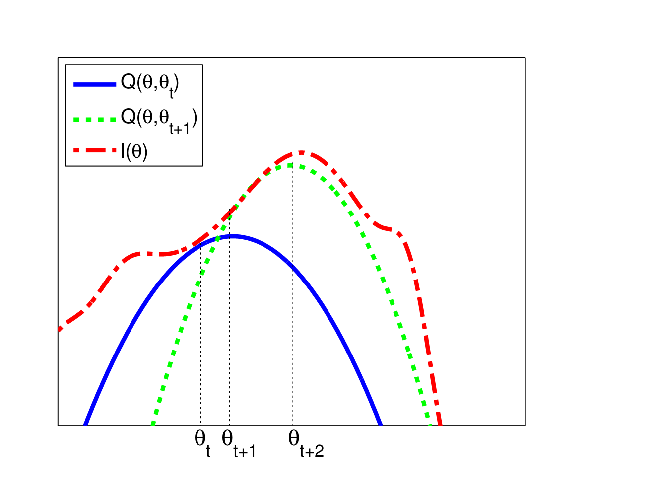 위 그림에서와 같이, $t$ 시점에서의 값 $\theta_{t}$ 에서의 surrogate function(파란색)을 찾고,해당 function을 최대로 하는 $\theta$를 다음 step의 값으로 설정하는 과정을 반복하면 함수의 local maximum과 local maximum에 대응하는 parameter를 찾을 수 있다.
Surrogate function을 찾는 방법에는 여러 가지 방법이 있을 수 있으나, 가장 쉽게 생각하면 Taylor expansion을 활용하여 구할 수 있다. 다음과 같은 Taylor expansion을 생각해보자.
\[l(\theta) = l(\theta^{t})+(\theta-\theta^{t})^{T}g(\theta^{t})+\frac{1}{2}(\theta-\theta^{t})^TH(\theta-\theta^{t})\]여기서 g는 gradient vector, H는 Hessian matrix를 각각 의미한다. 그러면 위 taylor expansion으로부터 다음을 만족하는 negative definite matrix $B$를 찾을 수 있다.
\[l(\theta) \geq l(\theta^{t})+(\theta-\theta^{t})^{T}g(\theta^{t})+\frac{1}{2}(\theta-\theta^{t})^TB(\theta-\theta^{t})\]이때 위 식의 좌변은 $\theta$에 대한 함수이므로, 우변의 함수를 $\theta$에 대한 것으로 간추리면 이로부터 다음과 같이 surrogate function을 도출할 수 있다.
\[Q(\theta,\theta^{t})=\theta^T(g(\theta^{t})-B\theta^{t})+\frac{1}{2}\theta^{T}B\theta\]또한, 위 surrogate function을 최대화하기 위해 $\theta$에 대해 미분하여 0이 되도록 하는 값을 찾으면 update 과정은 다음과 같이 나타난다.
\[\theta^{t+1}=\theta^{t}-B^{-1}g(\theta^{t})\]Ex. Logistic Regression
Binary logistic regression에서 앞서 살펴본 MM algorithm이 어떻게 적용되는지 살펴보자. 우선 n번째 sample이 class $c\in \lbrace 1,2\rbrace $ 에 포함될 확률은 각각
\[p(y_{n}=c\vert x_{n},w)=\frac{\exp(w_{c}^{T}x_n)}{\exp(w_{1}^{T}x_n)+\exp(w_{2}^{T}x_n)}\]으로 주어진다. 이때 normalization condition, 즉 두 클래스에 속할 확률의 합이 1이라는 조건에 의해 $w_{2}=0$으로 두고 하나의 weight parameter만 구해도 무방하다. 이를 이용해 로그가능도를 구하면 다음과 같다.
\[l(\theta\vert Y) = \sum_{n=1}^{N}\bigg[ y_{n1}w^{T}x_{n}-\log \big(1+\exp(w^{T}x_{n})\big) \bigg]\]여기서 $y_{n1}$은 $n$번째 관측치가 class 1인 경우 1의 값을 갖고 class 2인 경우 0의 값을 갖는다. 이를 바탕으로 Gradient를 구하면
\[\begin{aligned} g^{t}&= \nabla l(w^{t}) = X^{T}(y-\mu^{t})\\ \mu^{t}&= [p_{n}(w^{t}), 1-p_{n}(w^{t})]_{n=1}^{N} \end{aligned}\]과 같다. 또한, Hessian matrix의 lower bound는 다음과 같이 구해진다.
\[\begin{aligned} H(w)&= -\sum_{n=1}^{N}(\mathrm{diag}(p_{n}(w))-p_{n}(w)p_{n}(w)^{T})\otimes(x_{n}x_{n}^{T})\\ &> -\frac{1}{2}(1- \frac{1}{2})(\sum_{n=1}^{N}x_{n}^Tx_{n})\\ &= - \frac{1}{4}X^{T}X \end{aligned}\]이를 바탕으로 계산한 Logistic Regression에서의 MM updating algorithm은 다음과 같다.
\[w^{t+1}= w^{t}-4(X^{T}X)^{-1}g^{t}\]반면, IRLS(Iteratively reweighted Least Squares)로 구한 Updating algorithm은 다음과 같은데, 이를 비교해보면 MM algorithm에서의 inverse term은 단 한번만 계산해도 사용가능하므로 IRLS에 비해 전체적인 계산 속도가 빠를 수 밖에 없음을 확인할 수 있다.
\[\begin{aligned} w^{t+1}&= w^{t}-(X^{T}S^{t}X)^{-1}g^{t}\\ S^{t}&= \mathrm{diag}(\mu^{t}\odot (1-\mu^{t})) \end{aligned}\]Practice
Binary logistic regression에 대한 MM algorithm, IRLS algorithm을 직접 코드로 작성하여 실행해본 결과 속도차이를 확인할 수 있었다.
# MM algorithm for binary logistic regression

def MM(X, y, max_iter=1000, tol=1e-6):

    start_time = time.time()
    n, p = X.shape
    beta = np.zeros(p)
    Hessian = 4 * np.linalg.inv(X.T @ X)

    for i in range(max_iter):

        eta = X @ beta
        mu = np.exp(eta) / (1 + np.exp(eta))
        gradient = X.T @ (y - mu)
        beta_new = beta + Hessian @ gradient

        if np.linalg.norm(beta_new - beta) < tol:
            break

        beta = beta_new

    return beta, time.time() - start_time

beta_hat_MM, time_MM = MM(X, y)
# Compare with iterative reweighted least squares

def IRLS(X, y, max_iter=1000, tol=1e-6):

    start_time = time.time()

    n, p = X.shape

    beta = np.zeros(p)


    for i in range(max_iter):

        eta = X @ beta
        mu = np.exp(eta) / (1 + np.exp(eta))
        W = np.diag(mu * (1 - mu))
        Hessian = X.T @ W @ X
        gradient = X.T @ (y - mu)
        beta_new = beta + np.linalg.inv(Hessian) @ gradient

        if np.linalg.norm(beta_new - beta) < tol:
        end_time = time.time()
        break

    beta = beta_new

    return beta, end_time - start_time


beta_hat_IRLS, time_IRLS = IRLS(X, y)
print('MM algorithm: ', time_MM)
print('IRLS: ', time_IRLS)
# Result
# MM algorithm: 0.17301678657531738 IRLS: 1.429758071899414
References
- Probabilistic Machine Learning : Advanced Topics - K.Murphy
- Code on github : https://github.com/ddangchani/Velog/blob/main/Statistical%20Learning/MM%20algorithm.ipynb
Leave a comment